tebsorflow2.0 语义分割(Oxford-IIIT数据集)
语义分割是在像素级别上的分类,属于同一类的像素都要被归为一类,因此语义分割是从像素级别来理解图像的。The Oxford-IIIT Pet Dataset是一个宠物图像数据集,包含37种宠物,每种宠物200张左右宠物图片,并同时包含宠物轮廓标注信息。下面就是tensorflow2.0的对该数据集的语义分割实现。本文基于TF2.0 , 谷歌Colab平台。

from google.colab import drive
drive.mount('/content/gdrive')
import os
os.chdir("/content/gdrive/My Drive/Colab Notebooks/tensorflow")
Mounted at /content/gdrive
1.导入相关的包
import tensorflow as tf
import matplotlib.pyplot as plt
import numpy as np
import os

import glob
tf.__version__
'2.2.0'
2.数据的预处理
首先我们打印出一个图片和对应的分割图象
print(os.listdir("./DS/the-oxfordiiit-pet-dataset/annotations/annotations/trimaps/")[-5:])
img = tf.io.read_file("./DS/the-oxfordiiit-pet-dataset/annotations/annotations/trimaps/yorkshire_terrier_99.png")
img = tf.image.decode_png(img)
img = tf.squeeze(img)
plt.imshow(img)
['._Bombay_27.png', '._Birman_91.png', '._Bombay_154.png', '._Bombay_22.png', '._Birman_93.png']
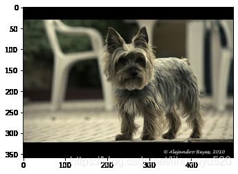
img1 = tf.io.read_file("./DS/the-oxfordiiit-pet-dataset/images/images/yorkshire_terrier_99.jpg")
img1 = tf.image.decode_png(img1)
plt.imshow(img1)

其次我们读取图片的路径和分割图片的的路径,并对其排序保证其一一对应,并随机打乱
#读取所有的图片
images = glob.glob("./DS/the-oxfordiiit-pet-dataset/images/images/*.jpg")
print(len(images))
anno = glob.glob("./DS/the-oxfordiiit-pet-dataset/annotations/annotations/trimaps/*.png")
print(len(anno))

images.sort(key=lambda x :x.split("\\")[-1].split(".jpg")[0])
anno.sort(key=lambda x :x.split("\\")[-1].split(".png")[0])
#打乱
np.random.seed(2019)
index = np.random.permutation(len(images))
images = np.array(images)[index]
anno = np.array(anno)[index]
7390 7390
构建图片载入方法,主要包括读取原图像(jpg格式),分割图像(png格式),归一化函数和图像载入四个函数
def read_jpg(path):
    img = tf.io.read_file(path)
    img = tf.image.decode_jpeg(img,channels=3)
    return img

def read_png(path):
    img = tf.io.read_file(path)
    img = tf.image.decode_png(img,channels=1)
    return img

# 归一化函数
def normal_img(input_images,input_anno):
    input_images = tf.cast(input_images,tf.float32)
    input_images = input_images/127.5 - 1
    input_anno = input_anno -1
    return input_images,input_anno

def load_image(input_images_path,input_anno_path):
    input_images = read_jpg(input_images_path)
    input_anno = read_png(input_anno_path)
    input_images = tf.image.resize(input_images,(224,224))
    input_anno = tf.image.resize(input_anno,(224,224))
    return normal_img(input_images,input_anno)
构建训练集和测试集,训练集的大小占总数据集的80%,bachsize=8,训练集有样本5912个,测试集有样本1478个。
AUTOTUNE = tf.data.experimental.AUTOTUNE
dataset = tf.data.Dataset.from_tensor_slices((images,anno))
dataset = dataset.map(load_image,num_parallel_calls=AUTOTUNE)
#%%设置训练数据和验证集数据的大小
test_count = int(len(images)*0.2)
train_count = len(images) - test_count
print(test_count,train_count)
#跳过test_count个
train_dataset = dataset.skip(test_count)
test_dataset = dataset.take(test_count)

batch_size = 8
# 设置一个和数据集大小一致的 shuffle buffer size(随机缓冲区大小)以保证数据被充分打乱。
train_ds = train_dataset.shuffle(buffer_size=train_count).repeat().batch(batch_size)
train_ds = train_ds.prefetch(buffer_size=tf.data.experimental.AUTOTUNE)
test_ds = test_dataset.batch(batch_size)
test_ds = test_ds.prefetch(buffer_size=tf.data.experimental.AUTOTUNE)
1478 5912
图片载入可视化实例
for image,anno in train_ds.take(1):
    plt.subplot(1,2,1)
    plt.imshow(tf.keras.preprocessing.image.array_to_img(image[0]))
    plt.subplot(1,2,2)
    plt.imshow(tf.keras.preprocessing.image.array_to_img(anno[0]))

3.模型构建与训练
我们采用的VGG16作为预训练模型,输入的图像为(224,224,3),采用全卷积网络(fully convolutional network,FCN)实现了从图像像素到像素类别的变换。与之前介绍的卷积神经网络有所不同,全卷积网络通过转置卷积(transposed convolution)层将中间层特征图的高和宽变换回输入图像的尺寸,从而令预测结果与输入图像在空间维(高和宽)上一一对应:给定空间维上的位置,通道维的输出即该位置对应像素的类别预测。
vgg16 = tf.keras.applications.VGG16(input_shape=(224, 224, 3),
                          include_top=False,
                          weights='imagenet')
vgg16.summary()
Model: "vgg16"
_________________________________________________________________
Layer (type)                 Output Shape              Param #
=================================================================
input_5 (InputLayer)         [(None, 224, 224, 3)]     0
_________________________________________________________________
block1_conv1 (Conv2D)        (None, 224, 224, 64)      1792
_________________________________________________________________
block1_conv2 (Conv2D)        (None, 224, 224, 64)      36928
_________________________________________________________________
block1_pool (MaxPooling2D)   (None, 112, 112, 64)      0
_________________________________________________________________
block2_conv1 (Conv2D)        (None, 112, 112, 128)     73856
_________________________________________________________________
block2_conv2 (Conv2D)        (None, 112, 112, 128)     147584
_________________________________________________________________
block2_pool (MaxPooling2D)   (None, 56, 56, 128)       0
_________________________________________________________________
block3_conv1 (Conv2D)        (None, 56, 56, 256)       295168
_________________________________________________________________
block3_conv2 (Conv2D)        (None, 56, 56, 256)       590080
_________________________________________________________________
block3_conv3 (Conv2D)        (None, 56, 56, 256)       590080
_________________________________________________________________
block3_pool (MaxPooling2D)   (None, 28, 28, 256)       0
_________________________________________________________________
block4_conv1 (Conv2D)        (None, 28, 28, 512)       1180160
_________________________________________________________________
block4_conv2 (Conv2D)        (None, 28, 28, 512)       2359808
_________________________________________________________________
block4_conv3 (Conv2D)        (None, 28, 28, 512)       2359808
_________________________________________________________________
block4_pool (MaxPooling2D)   (None, 14, 14, 512)       0
_________________________________________________________________
block5_conv1 (Conv2D)        (None, 14, 14, 512)       2359808
_________________________________________________________________
block5_conv2 (Conv2D)        (None, 14, 14, 512)       2359808
_________________________________________________________________
block5_conv3 (Conv2D)        (None, 14, 14, 512)       2359808
_________________________________________________________________
block5_pool (MaxPooling2D)   (None, 7, 7, 512)         0
=================================================================
Total params: 14,714,688
Trainable params: 14,714,688
Non-trainable params: 0
_________________________________________________________________
我们定义的一个上采样的计算块
class Connect(tf.keras.layers.Layer):
    def __init__(self,
               filters=256,
               name='Connect',
               **kwargs):
        super(Connect, self).__init__(name=name, **kwargs)

        self.Conv_Transpose = tf.keras.layers.Convolution2DTranspose(filters=filters,
                                                                    kernel_size=3,
                                                                    strides=2,
                                                                    padding="same",
                                                                    activation="relu")

        self.conv_out = tf.keras.layers.Conv2D(filters=filters,
                                           kernel_size=3,
                                           padding="same",
                                           activation="relu")
    def call(self, inputs):
        x = self.Conv_Transpose(inputs)
        return self.conv_out(x)
为了提取更为一般的特征我们将vgg13网络的"block5_conv3","block4_conv3","block3_conv3",等不同深度层输出结果进行了跳级(skip)连接。
layer_names = ["block5_conv3",
               "block4_conv3",
               "block3_conv3",
               "block5_pool"]
#得到4个输出
layers_out = [vgg16.get_layer(layer_name).output for layer_name in layer_names]
multi_out_model = tf.keras.models.Model(inputs = vgg16.input,
                                        outputs = layers_out)
multi_out_model.trainable = False

#创建输入
inputs = tf.keras.layers.Input(shape=(224,224,3))
out_block5_conv3,out_block4_conv3,out_block3_conv3,out = multi_out_model(inputs)
print(out_block5_conv3.shape)

x1 = Connect(512,name="connect_1")(out)
x1 = tf.add(x1,out_block5_conv3)#元素对应相加

x2 = Connect(512,name="connect_2")(x1)
x2 = tf.add(x2,out_block4_conv3)#元素对应相加

x3 = Connect(256,name="connect_3")(x2)
x3 = tf.add(x3,out_block3_conv3)#元素对应相加

x4 = Connect(128,name="connect_4")(x3)

prediction = tf.keras.layers.Convolution2DTranspose(filters=3,
                            kernel_size=3,
                            strides=2,
                            padding="same",
                            activation="softmax")(x4)

model = tf.keras.models.Model(inputs=inputs,outputs=prediction)
model.summary()
Model: "model_5"
__________________________________________________________________________________________________
Layer (type)                    Output Shape         Param #     Connected to
==================================================================================================
input_6 (InputLayer)            [(None, 224, 224, 3) 0
__________________________________________________________________________________________________
model_4 (Model)                 [(None, 14, 14, 512) 14714688    input_6[0][0]
__________________________________________________________________________________________________
connect_1 (Connect)             (None, 14, 14, 512)  4719616     model_4[1][3]
__________________________________________________________________________________________________
tf_op_layer_Add_6 (TensorFlowOp [(None, 14, 14, 512) 0           connect_1[0][0]
                                                                 model_4[1][0]
__________________________________________________________________________________________________
connect_2 (Connect)             (None, 28, 28, 512)  4719616     tf_op_layer_Add_6[0][0]
__________________________________________________________________________________________________
tf_op_layer_Add_7 (TensorFlowOp [(None, 28, 28, 512) 0           connect_2[0][0]
                                                                 model_4[1][1]
__________________________________________________________________________________________________
connect_3 (Connect)             (None, 56, 56, 256)  1769984     tf_op_layer_Add_7[0][0]
__________________________________________________________________________________________________
tf_op_layer_Add_8 (TensorFlowOp [(None, 56, 56, 256) 0           connect_3[0][0]
                                                                 model_4[1][2]
__________________________________________________________________________________________________
connect_4 (Connect)             (None, 112, 112, 128 442624      tf_op_layer_Add_8[0][0]
__________________________________________________________________________________________________
conv2d_transpose_14 (Conv2DTran (None, 224, 224, 3)  3459        connect_4[0][0]
==================================================================================================
Total params: 26,369,987
Trainable params: 11,655,299
Non-trainable params: 14,714,688
__________________________________________________________________________________________________
model.compile(optimizer=tf.keras.optimizers.Adam(learning_rate=0.0001),
        loss="sparse_categorical_crossentropy",
        metrics=["acc"]
       )

steps_per_eooch = train_count//batch_size
validation_steps = test_count//batch_size

history = model.fit(train_ds,
            epochs=3,
            steps_per_epoch=steps_per_eooch,
            validation_data=test_ds,
            validation_steps=validation_steps)
Epoch 1/3
739/739 [==============================] - 293s 396ms/step - loss: 0.3794 - acc: 0.8461 - val_loss: 0.2967 - val_acc: 0.8797
Epoch 2/3
739/739 [==============================] - 292s 395ms/step - loss: 0.2823 - acc: 0.8848 - val_loss: 0.2743 - val_acc: 0.8897
Epoch 3/3
739/739 [==============================] - 292s 395ms/step - loss: 0.2572 - acc: 0.8947 - val_loss: 0.2631 - val_acc: 0.8935
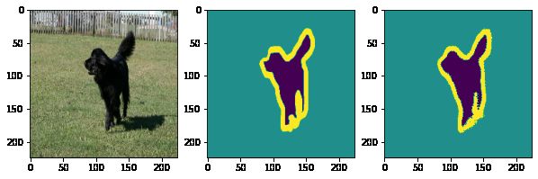
4. 模型评估
从上面的训练中,我们迭代了三次就达到了,达到90%的准确率,从整体说效果是不错的,下面我们可视化一个图像,观察具体的预测效果。
for image,mask in test_ds.take(1):
  pred_mask = model.predict(image)
  pred_mask = tf.argmax(pred_mask,axis=-1)
  pred_mask = pred_mask[...,tf.newaxis]
  plt.figure(figsize=(10,10))
  plt.subplot(1,3,1)
  plt.imshow(tf.keras.preprocessing.image.array_to_img(image[0]))
  plt.subplot(1,3,2)
  plt.imshow(tf.keras.preprocessing.image.array_to_img(mask[0]))
  plt.subplot(1,3,3)
  plt.imshow(tf.keras.preprocessing.image.array_to_img(pred_mask[0]))