计算机视觉：Bag of words算法实现图像识别与搜索

原理

综述

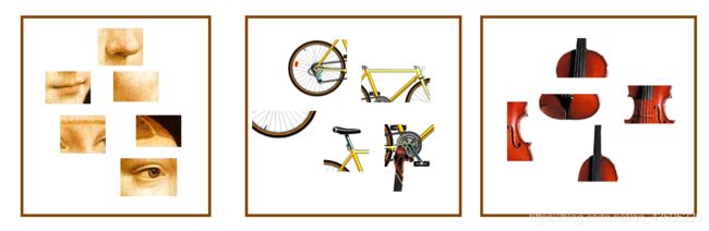
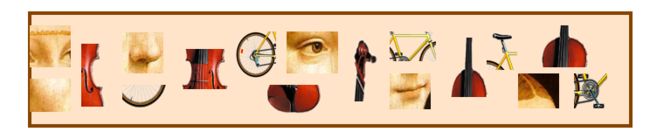
Bag of words，顾名思义，就是单词袋模型。这里的“单词”指代我们在图像数据库中所提取出的“图像特征”，每个特征就是一个单词，如下图所示。我们主要通过匹配图像中出现单词频率“最像”的图像，为其匹配图像。通过获取到的单词直方图，计算其与数据库中图像的欧氏距离，规定一定阈值内的图像为其所匹配到的图像，最终实现图像识别与搜索。

基础流程

1.特征提取
如下图所示，提取数据图像中的每个特征点即sift特征点。

2.学习 “视觉词典”
将所有提取到的特征点进行归类，获得“单词”，将所有的单词整合为一份“视觉词典”

3.数据量化
针对所输入的图片数据特征集，根据所得到的视觉词典对其进行量化

4.词频统计
将输入的图片数据转化为视觉单词的频率直方图

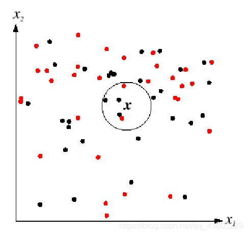
5.聚类
对图像进行聚类，可以使用K-means算法
首先随机初始化 K 个聚类中心，接着对应每个特征，根据距离关系赋值给某个中心/类别，再对每个类别，根据其对应的特征集重新计算聚类中心，重复该过程直值算法收敛，完成聚类。
在聚类过程中，可以通过给定输入图像的BOW直方图, 在数据库中查找 k 个最近邻的图像，可以根据这k个近邻图像的分类标签，进行投票获得分类结果。

结果与解析

数据集

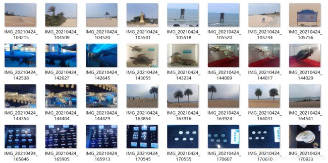
本文所用数据集为实地拍摄的厦门市各自然景区与博物馆场景图片数据，经Photoshop处理统一格式为 500X376大小的JPG图片，共130张，部分图片数据如下图

经过特征提取等处理后生成的数据库如下图，用于记录图片数据的名称，特征匹配值地址等数据

结果与解析

通过该算法，我们实现了输入一张图片找到数据集中多张与其类似的图片。
所得结果如下图所示，其中第一张图片为输入图片，2至5张为匹配后所得到的图片，从图中可以看出其成功匹配出了多张该沙滩的图片，但是也会出现最后一张丽龟标本图所示毫不相干的图片。这是由于该算法应用sift特征取过程中可能会出现错误的特征匹配，而在后续进行图片搜索，进行特征直方图对比过程中就会出现错配。但由于只是局部错配，因此在进行重排后其特征匹配的比率会低于像第二张图片这样与输入图片相似的图片数据。

同时，打开训练数据集，我们会发现里面有多张该沙滩的图片，但是却未能够进行正确的匹配，对于这一点我还有一些疑惑，个人觉得可能是由于沙滩的特征比较难提取，角点较少，且无法提取到关键区域的特征点多导致。

接着通过匹配灰鲸标本图片，并输入9张类似图片。可以发现所匹配的图像基本都是准确的，或是像最后几张图一般轮廓大致相似的图片，出现少量差别较大图片原因如上文所述。而对于下图所示出现轮廓相似的图片。个人认为是由于在将特征识别并汇入词典时都是应用灰度图的形式，因此可能会将不同颜色的特征单词识别为同一个单词，从而造成的特征匹配错误。

总结

问题	原因	解决方案
大差异图像错配	sift特征识别问题
相似图像未匹配	图像景物单一，特征重复
同轮廓图像错配	灰度图问题	改为RGB格式词典

源代码

1.生成词汇表

import pickle
from PCV.imagesearch import vocabulary
from PCV.tools.imtools import get_imlist
from PCV.localdescriptors import sift
from PCV.imagesearch import imagesearch
from PCV.geometry import homography
from sqlite3 import dbapi2 as sqlite


#获取图像列表
imlist = get_imlist('datasets/')
nbr_images = len(imlist)
#获取特征列表
featlist = [imlist[i][:-3]+'sift' for i in range(nbr_images)]

#提取文件夹下图像的sift特征
for i in range(nbr_images):
    sift.process_image(imlist[i], featlist[i])

#生成词汇
voc = vocabulary.Vocabulary('ukbenchtest')
voc.train(featlist, 888, 10) # 使用k-means算法在featurelist里边训练处一个词汇
                             # 注意这里使用了下采样的操作加快训练速度
                             # 将描述子投影到词汇上，以便创建直方图
#保存词汇
# saving vocabulary
with open('BOW/vocabulary.pkl', 'wb') as f:
    pickle.dump(voc, f)
print ('vocabulary is:', voc.name, voc.nbr_words)

2.生成数据库

import pickle
from PCV.imagesearch import vocabulary
from PCV.tools.imtools import get_imlist
from PCV.localdescriptors import sift
from PCV.imagesearch import imagesearch
from PCV.geometry import homography
from sqlite3 import dbapi2 as sqlite # 使用sqlite作为数据库


#获取图像列表
imlist = get_imlist('datasets/')
nbr_images = len(imlist)
#获取特征列表
featlist = [imlist[i][:-3]+'sift' for i in range(nbr_images)]

# load vocabulary
#载入词汇
with open('BOW/vocabulary.pkl', 'rb') as f:
    voc = pickle.load(f)
#创建索引
indx = imagesearch.Indexer('testImaAdd.db',voc) # 在Indexer这个类中创建表、索引，将图像数据写入数据库
indx.create_tables() # 创建表
# go through all images, project features on vocabulary and insert
#遍历所有的图像，并将它们的特征投影到词汇上
for i in range(nbr_images)[:888]:
    locs,descr = sift.read_features_from_file(featlist[i])
    indx.add_to_index(imlist[i],descr) # 使用add_to_index获取带有特征描述子的图像，投影到词汇上
                                       # 将图像的单词直方图编码存储
# commit to database
#提交到数据库
indx.db_commit()

con = sqlite.connect('testImaAdd.db')
print (con.execute('select count (filename) from imlist').fetchone())
print (con.execute('select * from imlist').fetchone())

3.图像搜索

# -*- coding: utf-8 -*- 
#使用视觉单词表示图像时不包含图像特征的位置信息
import pickle
from PCV.localdescriptors import sift
from PCV.imagesearch import imagesearch
from PCV.geometry import homography
from PCV.tools.imtools import get_imlist

# load image list and vocabulary
#载入图像列表
#imlist = get_imlist('E:/Python37_course/test7/first1000/')
imlist = get_imlist('datasets/')
nbr_images = len(imlist)
#载入特征列表
featlist = [imlist[i][:-3]+'sift' for i in range(nbr_images)]

#载入词汇
'''with open('E:/Python37_course/test7/first1000/vocabulary.pkl', 'rb') as f:
    voc = pickle.load(f)'''
with open('BOW/vocabulary.pkl', 'rb') as f:
    voc = pickle.load(f)

src = imagesearch.Searcher('testImaAdd.db',voc)# Searcher类读入图像的单词直方图执行查询

# index of query image and number of results to return
#查询图像索引和查询返回的图像数
q_ind = 0
nbr_results = 130

# regular query
# 常规查询(按欧式距离对结果排序)
res_reg = [w[1] for w in src.query(imlist[q_ind])[:nbr_results]] # 查询的结果 
print ('top matches (regular):', res_reg)

# load image features for query image
#载入查询图像特征进行匹配
q_locs,q_descr = sift.read_features_from_file(featlist[q_ind])
fp = homography.make_homog(q_locs[:,:2].T)

# RANSAC model for homography fitting
#用单应性进行拟合建立RANSAC模型
model = homography.RansacModel()
rank = {
     }
# load image features for result
#载入候选图像的特征
for ndx in res_reg[1:]:
    try:
        locs,descr = sift.read_features_from_file(featlist[ndx]) 
    except:
        continue

    #locs,descr = sift.read_features_from_file(featlist[ndx])  # because 'ndx' is a rowid of the DB that starts at 1
    # get matches
    matches = sift.match(q_descr,descr)
    ind = matches.nonzero()[0]
    ind2 = matches[ind]
    tp = homography.make_homog(locs[:,:2].T)
    # compute homography, count inliers. if not enough matches return empty list
    # 计算单应性矩阵
    try:
        H,inliers = homography.H_from_ransac(fp[:,ind],tp[:,ind2],model,match_theshold=4)
    except:
        inliers = []
    # store inlier count
    rank[ndx] = len(inliers)

# sort dictionary to get the most inliers first
# 对字典进行排序，可以得到重排之后的查询结果
sorted_rank = sorted(rank.items(), key=lambda t: t[1], reverse=True)
res_geom = [res_reg[0]]+[s[0] for s in sorted_rank]
print ('top matches (homography):', res_geom)

# 显示查询结果
imagesearch.plot_results(src,res_reg[:6]) #常规查询
imagesearch.plot_results(src,res_geom[:6]) #重排后的结果

出现的错误及解决方案

https://blog.csdn.net/qq_43605229/article/details/117608008