【论文翻译】Mean Shift: A Robust Approach toward Feature Space Analysis

论文题目：Mean Shift: A Robust Approach toward Feature Space Analysis
论文来源: Mean Shift: A Robust Approach toward Feature Space Analysis
翻译人：BDML@CQUT实验室

Mean Shift: A Robust Approach toward Feature Space Analysis

均值偏移：面向特征空间分析的鲁棒性方法

$$DorinComanici{u}^{1}PeterMee{r}^2$$

$$\begin{gathered} {}^{1}SiemensCorporateResearch \\ 755CollegeRoadEast,Princeton,NJ08540 \\ comanici@scr.siemens.com \end{gathered}$$

$$\begin{gathered} {}^{2}ElectricalandComputerEngineeringDepartment \\ RutgersUniversity \\ 94BrettRoad,Piscataway,NJ08854-8058 \\ meer@caip.rutgers.edu \end{gathered}$$

Abstract

A general nonparametric technique is proposed for the analysis of a complex multimodal feature space and to delineate arbitrarily shaped clusters in it. The basic computational module of the technique is an old pattern recognition procedure, the mean shift. We prove for discrete data the convergence of a recursive mean shift procedure to the nearest stationary point of the underlying density function and thus its utility in detecting the modes of the density. The equivalence of the mean shift procedure to the Nadaraya–Watson estimator from kernel regression and the robust M-estimators of location is also established. Algorithms for two low-level vision tasks, discontinuity preserving smoothing and image segmentation are described as applications. In these algorithms the only user set parameter is the resolution of the analysis, and either gray level or color images are accepted as input. Extensive experimental results illustrate their excellent performance.

Keywords: mean shift; clustering; image segmentation; image smoothing; feature space; low-level
vision

摘要

本文提出了一种通用的非参数技术，用于分析复杂的多峰特征空间并在其中描绘任意形状的聚类。该技术的基本计算模块是一个古老的模式识别程序，均值偏移。对于离散数据，我们证明了递归均值偏移过程收敛到基础密度函数的最近固定点，从而证明了其在检测密度模式中的效用。还建立了通过核回归和位置的鲁棒M估计到Nadaraya–Watson估计的均值偏移过程的等价性。描述了用于两个底层视觉任务的算法，即图像平滑和图像分割。在这些算法中，唯一的用户设置参数是分析的分辨率，并且可以接受灰度或彩色图像作为输入。大量的实验结果证明了它们的出色性能。

关键字：均值偏移；聚类；图像分割；图像平滑；特征空间；底层视觉

1 Introduction

Low-level computer vision tasks are misleadingly difficult. Incorrect results can be easily obtained since the employed techniques often rely upon the user correctly guessing the values for the tuning parameters. To improve performance the execution of low-level tasks should be task driven, i.e., supported by independent high level information. This approach, however, requires that first the low-level stage provides a reliable enough representation of the input, and that the feature extraction process is controlled only by very few tuning parameters corresponding to intuitive measures in the input domain.

Feature space based analysis of images is a paradigm which can achieve the above stated goals. A feature space is a mapping of the input obtained through the processing of the data in small subsets at a time. For each subset a parametric representation of the feature of interest is obtained and the result is mapped into a point in the multidimensional space of the parameter. After the entire input is processed, significant features correspond to denser regions in the feature space, i.e., to clusters, and the goal of the analysis is the delineation of these clusters.

The nature of the feature space is application dependent. The subsets employed in the mapping can range from individual pixels as in the color space representation of an image, to a set of quasi-randomly chosen data points as in the probabilistic Hough transform. Both the advantage and the disadvantage of the feature space paradigm are arising from the global nature of the derived representation of the input. On one hand, all the evidence for the presence of a significant feature is pooled together providing an excellent tolerance to a noise level which may render local decisions unreliable. On the other hand, features with lesser support in the feature space may not be detected in spite of being salient for the task to be executed. This disadvantage, however, can be largely avoided by either augmenting the feature space with additional (spatial) parameters from the input domain, or by robust post processing of the input domain guided by the results of the feature space analysis.

Analysis of the feature space is application independent. While there are a plethora of published clustering techniques, most of them are not adequate to analyze feature spaces derived from real data. Methods which rely upon a priori knowledge of the number of clusters present (including those which use optimization of a global criterion to find this number), as well as methods which implicitly assume the same shape (most often elliptical) for all the clusters in the space, are not able to handle the complexity of a real feature space. For a recent survey of such methods see [29, Sec.8].

In Figure 1 a typical example is shown. The color image in Figure 1a is mapped into the three-dimensional Luv color space (to be discussed in Section 4). There is a continuous transition between the clusters arising from the dominant colors, and a decomposition of the space into elliptical tiles will introduce severe artifacts. Enforcing a Gaussian mixture model over such data is doomed to fail, e.g., [49], and even the use of a robust approach with contaminated Gaussian densities [67] cannot be satisfactory for such complex cases. Note also that the mixture models require the number of clusters as a parameter which raises its own challenges. For example, the method described in [45] proposes several different ways to determine this number.

Arbitrarily structured feature spaces can be analyzed only by nonparametric methods since these methods do not have embedded assumptions. Numerous nonparametric clustering methods were described in the literature and they can be classified into two large classes: hierarchical clustering and density estimation. Hierarchical clustering techniques either aggregate or divide the data based on some proximity measure. See [28, Sec.3.2] for a survey of hierarchical clustering methods. The hierarchical methods tend to be computationally expensive and the definition of a meaningful stopping criterion for the fusion (or division) of the data is not straightforward.

The rationale behind the density estimation based nonparametric clustering approach is that the feature space can be regarded as the empirical probability density function (p.d.f.) of the represented parameter. Dense regions in the feature space thus correspond to local maxima of the p.d.f., that is, to the modes of the unknown density. Once the location of a mode is determined, the cluster associated with it is delineated based on the local structure of the feature space [25, 60, 63].

Our approach to mode detection and clustering is based on the mean shift procedure, proposed in 1975 by Fukunaga and Hostetler [21] and largely forgotten till Cheng’s paper [7] rekindled the interest in it. In spite of its excellent qualities, the mean shift procedure does not seem to be known in the statistical literature. While the book [54, Sec.6.2.2] discusses [21], the advantages of employing a mean shift type procedure in density estimation were only recently rediscovered [8].

As will be proven in the sequel a computational module based on the mean shift procedure is an extremely versatile tool for feature space analysis and can provide reliable solutions for many vision tasks. In Section 2 the mean shift procedure is defined and its properties are analyzed. In Section 3 the procedure is used as the computational module for robust feature space analysis and implementational issues are discussed. In Section 4 the feature space analysis technique is applied to two low level vision tasks: discontinuity preserving filtering and image segmentation. Both algorithms can have as input either gray level or color images and the only parameter to be tuned by the user is the resolution of the analysis. The applicability of the mean shift procedure is not restricted to the presented examples. In Section 5 other applications are mentioned and the procedure is put into a more general context.

1 引言

底层的计算机视觉任务具有误导性。由于所采用的技术通常依赖于用户正确猜测调整参数的值，因此很容易获得不正确的结果。为了提高性能，底层任务的执行应该由任务驱动，即由独立的高级信息支持。但是，这种方法要求首先底层阶段提供输入的足够可靠的表示，并且特征提取过程仅由很少的与输入域中的直观度量相对应的调整参数来控制。

基于特征空间的图像分析是可以实现上述目标的范例。特征空间是一次通过处理小子集中的数据获得的输入的映射。对于每个子集，获取感兴趣特征的参数表示，并将结果映射到参数多维空间中的一个点。在处理完所有输入之后，重要特征对应于特征空间中较密集的区域，即对应于聚类，而分析的目的是描绘这些聚类。

特征空间的性质取决于应用程序。映射中采用的子集的范围可以从图像颜色空间表示中的单个像素到概率霍夫变换中的一组准随机选择的数据点。特征空间范式的优势和劣势都源于输入的派生表示的全局性质。一方面，将存在重要特征的所有证据汇总在一起，以提供对噪声水平的出色容忍度，这可能会使本地决策变得不可靠。另一方面，尽管对要执行的任务很重要，但可能无法检测到在特征空间中支持较少的特征。但是，可以通过使用来自输入域的其他（空间）参数扩展特征空间，或通过特征空间分析的结果对输入域进行可靠的后处理，来很大程度上避免此缺点。

特征空间的分析与应用程序无关。尽管存在大量已发布的聚类技术，但大多数技术不足以分析从真实数据得出的特征空间。依赖于对存在的聚类数的先验知识的方法（包括那些使用全局准则优化来找到此数目的方法），以及隐含地假设空间中所有聚类的形状相同（通常为椭圆形）的方法不能处理真实特征空间的复杂性。有关此类方法的最新调查，请参见[29，第8节]。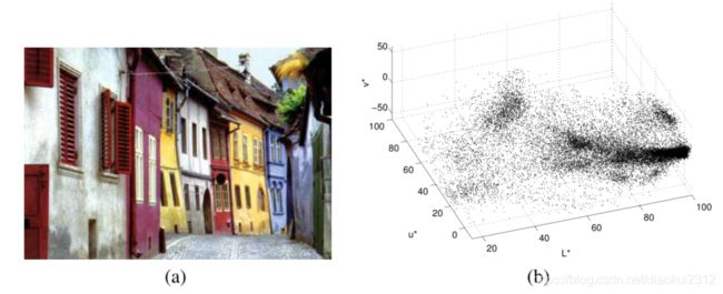

图1：一个特征空间的例子。（a）是一个400x276色彩的图像。（b）是相应的L*u*v色彩空间110，400个数据点

图1中显示了一个典型示例。图1a中的彩色图像被映射到三维L*u*v彩色空间（将在第4节中讨论）。由主要颜色引起的聚类之间存在连续过渡，并且空间分解为椭圆形瓷砖会引入严重的伪影。对此类数据执行高斯混合模型注定会失败，例如，[49]，甚至对于这种复杂情况，即使使用具有受污染的高斯密度的稳健方法[67]也无法令人满意。还要注意，混合模型需要将聚类数作为参数，这会带来挑战。例如，[45]中描述的方法提出了几种不同的方法来确定该数字。

任意结构化的特征空间只能通过非参数方法进行分析，因为这些方法没有嵌入的假设。文献中描述了许多非参数聚类方法，它们可分为两大类：层次聚类和密度估计。层次聚类技术基于某种接近度度量来聚合或划分数据。有关分层聚类方法的概述，请参见[28，第3.2节]。分层方法在计算上趋于昂贵，并且对于数据的融合（或划分）有意义的停止标准的定义并不简单。

基于密度估计的非参数聚类方法的基本原理是可以将特征空间视为所表示参数的经验概率密度函数（p.d.f.）。因此，特征空间中的密集区域对应于p.d.f.的局部最大值，即对应于未知密度的众数。一旦确定了模式的位置，便会基于特征空间的局部结构[25、60、63]来确定与其关联的群集。

我们的模式检测和聚类方法是基于均值偏移过程，1975年，Fukunaga和Hostetler[21]提出了这个想法，但大部分已经被遗忘，直到Cheng的论文[7]重新点燃了人们对它的兴趣。尽管具有出色的质量，但该均值偏移过程在统计文献中似乎并不为人所知。本书[54，Sec.6.2.2]讨论了[21]时，直到最近才重新发现在密度估计中采用均值偏移类型过程的优势[8]。

正如后续将证明的那样，基于均值偏移过程的计算模块是用于特征空间分析的极其通用的工具，可以为许多视觉任务提供可靠的解决方案。在第2节中，定义了均值偏移程序并分析了其性质。在第3节中，该过程用作鲁棒特征空间分析的计算模块，并讨论了实现问题。在第4节中，特征空间分析技术应用于两个底层视觉任务：不连续性保留过滤和图像分割。两种算法都可以输入灰度图像或彩色图像作为输入，并且用户要调整的唯一参数是分析的分辨率。均值偏移过程的适用性不限于所提供的示例。在第5节中，提到了其他应用程序，并且将该过程放到了更一般的上下文中。

2 The Mean Shift Procedure

Kernel density estimation (known as the Parzen window technique in the pattern recognition literature [17, Sec.4.3]) is the most popular density estimation method. Given $n$ data points $X_i$, $i=1,...,n$ in the $d$-dimensional space $R^d$, the multivariate kernel density estimator with kernel $K(X)$ and a symmetric positive definite $d\times d$ bandwidth matrix $H$, computed in the point $X$ is given by
$$\hat{f}(X)=\frac{1}{n}\sum _{i=1}^n{K}_H(X-X_i)\text{\hspace{1em}(1)}$$
where
$$K_H(X)=|H{|}^{-1/2}K(H^{-1/2}X)\text{\hspace{1em}(2)}$$
The $d$-variate kernel $K(X)$, is a bounded function with compact support satisfying [62, p.95]
$$\begin{gathered} {\int }_{R^d}K(X)dX=1\underset{||X||\to \infty }{\lim }||X|{|}^{d}k(X)=0 \\ {\int }_{R^d}XK(X)dX=0{\int }_{R^d}X{X}^{T}K(X)dX=c_{K}I \\ \text{\hspace{1em}(3)} \end{gathered}$$
where $c_K$ is a constant. The multivariate kernel can be generated from a symmetric univariate kernel $K_1(x)$ in two different ways
$$K^P(X)=\prod _{i=1}^d{K}_1(x_i)K^S(X)=a_{k,d}{K}_1(||X||)\text{\hspace{1em}(4)}$$
where $K^P(X)$ is obtained from the product of the univariate kernels, and $K^P(X)$ from rotating $K_1(x)$ in $R_d$, i.e., $K^S(X)$ is radially symmetric. The constant $a_{k,d}^{-1}={\int }_{R^d}{K}_1(||X||)dX$ assures that $K^S(X)$ integrates to one, though this condition can be relaxed in our context. Either type of multivariate kernel obeys (3), but for our purposes the radially symmetric kernels are often more suitable.

We are interested only in a special class of radially symmetric kernels satisfying
$$K(X)=c_{k,d}k(||X|{|}^2)\text{\hspace{1em}(5)}$$
in which case it suffices to define the function $k(x)$ called the profile of the kernel, only for $x\ge 0$.The normalization constant $c_{k,d}$, which makes $K(X)$to integrate to one, is assumed strictly positive.

Using a fully parameterized H increases the complexity of the estimation [62, p.106] and in practice the bandwidth matrix H is chosen either as diagonal H = diag$[h_1^2,...,h_d^2]$, or proportional to the identity matrix H = $h^2$ I. The clear advantage of the latter case is that only one bandwidth parameter $h>0$ must be provided, however, as can be seen from (2) then the validity of an Euclidean metric for the feature space should be confirmed first. Employing only one bandwidth parameter, the kernel density estimator (1) becomes the well known expression
$$\hat{f}(x)=\frac{1}{n{h}^d}\sum _{i=1}^{n}K(\frac{X-X_i}{h})\text{\hspace{1em}(6)}$$
The quality of a kernel density estimator is measured by the mean of the square error between the density and its estimate, integrated over the domain of definition. In practice, however, only an asymptotic approximation of this measure (denoted as AMISE) can be computed. Under the asymptotics the number of data points $n\to \infty$ while the bandwidth $h\to \infty$ at a rate slower than $n^{-1}$. For both types of multivariate kernels the AMISE measure is minimized by the Epanechnikov kernel [51, p.139], [62, p.104] having the profile
$$k_E(x)=\{\begin{array}{ll}1-x& 0\le x\le 1\\ 0& x>1\end{array}\text{\hspace{1em}(7)}$$
which yields the radially symmetric kernel
$$k_E(x)=\{\begin{array}{ll}\frac{1}{2}{c}_d^{-1}(d+2(1-||X|{|}^2))& ||X||\le 1\\ 0& otherwise\end{array}\text{\hspace{1em}(8)}$$
where $c_d$ is the volume of the unit $d$-dimensional sphere. Note that the Epanechnikov profile is not differentiable at the boundary. The profile
$$k_N(x)=\exp (-\frac{1}{2}x)x\ge 0\text{\hspace{1em}(9)}$$
yields the multivariate normal kernel
$$K_N(X)=(2\pi {)}^{-d/2}\exp (-\frac{1}{2}||X|{|}^2)\text{\hspace{1em}(10)}$$
for both types of composition (4). The normal kernel is often symmetrically truncated to have a
kernel with finite support.

While these two kernels will suffice for most applications we are interested in, all the results
presented below are valid for arbitrary kernels within the conditions to be stated. Employing the
profile notation the density estimator (6) can be rewritten as
$${\hat{f}}_{h,k}(X)=\frac{c_{k,d}}{n{h}^d}\sum _{i=1}^{n}k(||\frac{X-X_i}{h}|{|}^2)\text{\hspace{1em}(11)}$$
The first stepinthe analysisof a feature space withthe underlyingdensity $f(x)$ is to find themodes of this density. The modes are located among the zeros of the gradient $\nabla f(x)=0$, and the mean shift procedure is an elegant way to locate these zeros without estimating the density.

2 均值偏移步骤

内核密度估计（在模式识别文献中称为Parzen窗口技术[17，第4.3节]）是最流行的密度估计方法。给定$n$个数据点 $X_i$, $i=1,...,n$ 在$d$维空间$R^d$中，在点x上计算的具有核$K(X)$和对称正定$d\times d$ 带宽矩阵H的多元核密度估计器由下式给出：
$$\hat{f}(X)=\frac{1}{n}\sum _{i=1}^n{K}_H(X-X_i)\text{\hspace{1em}(1)}$$
则
$$K_H(X)=|H{|}^{-1/2}K(H^{-1/2}X)\text{\hspace{1em}(2)}$$
$d$变量内核$K(X)$是一个有界函数
$$\begin{gathered} {\int }_{R^d}K(X)dX=1\underset{||X||\to \infty }{\lim }||X|{|}^{d}k(X)=0 \\ {\int }_{R^d}XK(X)dX=0{\int }_{R^d}X{X}^{T}K(X)dX=c_{K}I \\ \text{\hspace{1em}(3)} \end{gathered}$$
其中$c$为常数。可以采用两种不同方式从对称单变量内核$K_1(x)$生成多变量内核
$$K^P(X)=\prod _{i=1}^d{K}_1(x_i)K^S(X)=a_{k,d}{K}_1(||X||)\text{\hspace{1em}(4)}$$
其中，$K^P(X)$是从单变量核的乘积获得的，而$K^R(X)$是通过在$R^d$中旋转$K_1(x)$来获得的，即$K^S(X)$是径向对称的。常数$a_{k,d}^{-1}={\int }_{R^d}{K}_1(||X||)dX$可以确保$K^S(X)$积分为1，不过在我们的上下文中可以放宽此条件。两种类型的多元核均服从（3），但出于我们的目的，径向对称核通常更适合。

我们只对满足以下条件的一类特殊的径向对称核感兴趣：
$$K(X)=c_{k,d}k(||X|{|}^2)\text{\hspace{1em}(5)}$$
在这种情况下，仅对于$x\ge 0$定义为内核轮廓的函数$k(x)$就足够了。使$K(X)$积分为1的归一化常数$c_{k,d}$严格地假定为正。

使用完全参数化的H会增加估计的复杂度[62，p.106]，实际上，带宽矩阵H可以选择为对角线H = diag$[h_1^2,...,h_d^2]$，或与恒等式H = $h^2$ I成正比。后一种情况的明显优势是，仅必须提供一个带宽参数$h>0$，但是，从（2）中可以看出有效性首先应确定特征空间的欧几里得度量。仅使用一个带宽参数，核密度估计器（1）成为众所周知的表达式
$$\hat{f}(x)=\frac{1}{n{h}^d}\sum _{i=1}^{n}K(\frac{X-X_i}{h})\text{\hspace{1em}(6)}$$
内核密度估计量的质量是通过在定义范围内积分的密度与其估计值之间的平方误差的平均值来衡量的。但是，实际上，只能计算该度量的渐近近似值（表示为AMISE）。在渐近状态下，数据点的数量为$n\to \infty$, 而带宽$h\to \infty$的速率慢于$ n^{-1}$。对于两种类型的多元内核，通过具有以下特征的Epanechnikov内核[51，p.139]，[62，p.104]可以将AMISE度量最小化
$$k_E(x)=\{\begin{array}{ll}1-x& 0\le x\le 1\\ 0& x>1\end{array}\text{\hspace{1em}(7)}$$
其中产生径向对称的内核
$$k_E(x)=\{\begin{array}{ll}\frac{1}{2}{c}_d^{-1}(d+2(1-||X|{|}^2))& ||X||\le 1\\ 0& otherwise\end{array}\text{\hspace{1em}(8)}$$
其中 $c$ 是单位 $d$ 维球体的体积。注意，Epanechnikov轮廓在边界处是不可微的。
$$k_N(x)=\exp (-\frac{1}{2}x)x\ge 0\text{\hspace{1em}(9)}$$
产生多元正态核
$$K_N(X)=(2\pi {)}^{-d/2}\exp (-\frac{1}{2}||X|{|}^2)\text{\hspace{1em}(10)}$$
对于两种类型的成分（4）。普通内核通常被对称地截断，以使内核具有有限的支持。

尽管这两个内核足以满足我们感兴趣的大多数应用程序的需要，但下面列出的所有结果对于在规定条件下的任意内核都是有效的。利用轮廓符号，密度估算器（6）可以重写为
$${\hat{f}}_{h,k}(X)=\frac{c_{k,d}}{n{h}^d}\sum _{i=1}^{n}k(||\frac{X-X_i}{h}|{|}^2)\text{\hspace{1em}(11)}$$
分析具有基础密度 $f(x)$ 的特征空间的第一步是找到该密度的模式。这些模式位于梯度 $\nabla f(x)=0$ 的零之间，并且均值偏移过程是一种无需估计密度即可找到这些零的绝妙方法。

2.1 Density Gradient Estimation

The density gradient estimator is obtained as the gradient of the density estimator by exploiting the
linearity of (11)
$$\widehat{\nabla f_{h,k}(X)}\equiv \nabla {\hat{f}}_{h,k}(X)=\frac{2c_{k,d}}{n{h}^{d+2}}\sum _{i=1}^n(X-X_i)k^{{}^{\prime }}\left({\Vert \frac{X-X_i}{h}\Vert }^2\right)\text{\hspace{1em}(12)}$$
We define the function
$$g(x)=-k^{{}^{\prime }}(x)\text{\hspace{1em}(13)}$$
assuming that the derivative of the kernel profile $k$ exists for all $x\in [0,\infty )$, except for a finite set of points. Using now $g(x)$ for profile, the kernel $G(X)$ is defined as
$$G(X)=c_{g,d}g(\Vert X{\Vert }^2)\text{\hspace{1em}(14)}$$
where $c_{g,d}$ is the corresponding normalization constant. The kernel $K(X)$ was called the shadow of $G(X)$ in [7] in a slightly different context. Note that the Epanechnikov kernel is the shadow of the uniform kernel, i.e., the $d$-dimensional unit sphere; while the normal kernel and its shadow have the same expression.

Introducing $g(x)$ into (12) yields
$$\begin{gathered} \hat{\nabla }{f}_{h,K}(X)=\frac{2c_{k,d}}{n{h}^{d+2}}\sum _{i=1}^n(X_i-X)g\left({\Vert \frac{X-X_i}{h}\Vert }^2\right) \\ =\frac{2c_{k,d}}{n{h}^{d+2}}\left[\sum _{i=1}^{n}g\left({\Vert \frac{X-X_i}{h}\Vert }^2\right)\right]\left[\frac{{\sum }_{i=1}^n{X}_{i}g\left({\Vert \frac{X-X_i}{h}\Vert }^2\right)}{{\sum }_{i=1}^{n}g\left({\Vert \frac{X-X_i}{h}\Vert }^2\right)}-x\right]\text{\hspace{1em}(15)} \end{gathered}$$
where ${\sum }_{i=1}^{n}g\left({\Vert \frac{X-X_i}{h}\Vert }^2\right)$ is assumed to be a positive number. This condition is easy to satisfy for all the profiles met in practice. Both terms of the product in (15) have special significance. From (11) the first term is proportional to the density estimate at $X$ computed with the kernel $G$
$${\hat{f}}_{h,G}(X)=\frac{c_{g,d}}{n{h}^d}\sum _{i=1}^{n}g\left({\Vert \frac{X-X_i}{h}\Vert }^2\right)\text{\hspace{1em}(16)}$$
The second term is the mean shift
$${m\text{m}m}_{h,G}(X)=\frac{{\sum }_{i=1}^n{X}_{i}g\left({\Vert \frac{X-X_i}{h}\Vert }^2\right)}{{\sum }_{i=1}^{n}g\left({\Vert \frac{X-X_i}{h}\Vert }^2\right)}-x\text{\hspace{1em}(17)}$$
i.e., the difference between the weighted mean, using the kernel $G$ for weights, and $X$ the center of the kernel (window). From (16) and (17) the expression (15) becomes
$$\hat{\nabla }{f}_{h,K}(X)={\hat{f}}_{h,G}(X)\frac{2c_{k,d}}{h^2{c}_{g,d}}{m\text{m}m}_{h,G}(X)\text{\hspace{1em}(18)}$$
yielding
$${m\text{m}m}_{h,G}(X)=\frac{1}{2}{h}^{2}c\frac{\hat{\nabla }{f}_{h,K}(X)}{\widehat{f_{h,G}}(X)}\text{\hspace{1em}(19)}$$
The expression (19) shows that at location $X$ the mean shift vector computed with kernel $G$ is proportional to the normalizeddensity gradient estimate obtained with kernel $K$. The normalization is by the density estimate in $X$ computed with the kernel $G$. The mean shift vector thus always points toward the direction of maximum increase in the density. This is a more general formulation of the property first remarked by Fukunaga and Hostetler [20, p.535], [21], and also discussed in [7].

The relation captured in (19) is intuitive,the local mean is shifted toward the region in which the majority of the points reside. Since the mean shift vector is aligned with the local gradient estimate it can define a path leading to a stationary point of the estimated density. The modes of the density are such stationary points. The mean shift procedure, obtained by successive

​ – computation of the mean shift vector ${m\text{m}m}_{h,G}(X)$,

​ – translation of the kernel (window) $G(X)$ by ${m\text{m}m}_{h,G}(X)$,

is guaranteed to converge at a nearby point where the estimate (11) has zero gradient, as will be shown in the next section. The presence of the normalization by the density estimate is a desirable feature. The regions of low density values are of no interest for the feature space analysis, and in such regions the mean shift steps are large. Similarly, near local maxima the steps are small, and the analysis more refined. The mean shift procedure thus is an adaptive gradient ascent method.

2.1 密度梯度估计

利用（11）的线性可将密度梯度估算器作为密度估算器的梯度获得
$$\widehat{\nabla f_{h,k}(X)}\equiv \nabla {\hat{f}}_{h,k}(X)=\frac{2c_{k,d}}{n{h}^{d+2}}\sum _{i=1}^n(X-X_i)k^{{}^{\prime }}\left({\Vert \frac{X-X_i}{h}\Vert }^2\right)\text{\hspace{1em}(12)}$$
令
$$g(x)=-k^{{}^{\prime }}(x)\text{\hspace{1em}(13)}$$
假设内核配置文件 $k$ 的导数对于所有 $x\in [0,\infty )$，但一组有限的点除外。现在使用 $g(x)$ 进行分析，将内核 $G(X)$ 定义为
$$G(X)=c_{g,d}g(\Vert X{\Vert }^2)\text{\hspace{1em}(14)}$$
其中 $c_{g,d}$ 是对应的归一化常数。在[7]中，内核 在$K(X)$ 稍微不同的上下文中称为 $G(X)$ 的阴影。请注意，Epanechnikov核是均匀核（即d维单位球体）的阴影；而普通内核及其阴影具有相同的表达。

将 $g(x)$ 带入(12)
$$\begin{gathered} \hat{\nabla }{f}_{h,K}(X)=\frac{2c_{k,d}}{n{h}^{d+2}}\sum _{i=1}^n(X_i-X)g\left({\Vert \frac{X-X_i}{h}\Vert }^2\right) \\ =\frac{2c_{k,d}}{n{h}^{d+2}}\left[\sum _{i=1}^{n}g\left({\Vert \frac{X-X_i}{h}\Vert }^2\right)\right]\left[\frac{{\sum }_{i=1}^n{X}_{i}g\left({\Vert \frac{X-X_i}{h}\Vert }^2\right)}{{\sum }_{i=1}^{n}g\left({\Vert \frac{X-X_i}{h}\Vert }^2\right)}-x\right]\text{\hspace{1em}(15)} \end{gathered}$$
假定 ${\sum }_{i=1}^{n}g\left({\Vert \frac{X-X_i}{h}\Vert }^2\right)$ 为正数，对于在实践中满足的所有配置文件，此条件很容易满足。(15）中产品的两个术语都具有特殊的意义。根据（11），第一项与使用核G计算的x处的密度估计值成比例
$${\hat{f}}_{h,G}(X)=\frac{c_{g,d}}{n{h}^d}\sum _{i=1}^{n}g\left({\Vert \frac{X-X_i}{h}\Vert }^2\right)\text{\hspace{1em}(16)}$$
第二项是均值偏移
$${m\text{m}m}_{h,G}(X)=\frac{{\sum }_{i=1}^n{X}_{i}g\left({\Vert \frac{X-X_i}{h}\Vert }^2\right)}{{\sum }_{i=1}^{n}g\left({\Vert \frac{X-X_i}{h}\Vert }^2\right)}-x\text{\hspace{1em}(17)}$$
即，使用内核 $G$ 进行加权的加权平均值与 $X$ 内核中心（窗口）之间的差。从（16）和（17）表达式（15）变为
$$\hat{\nabla }{f}_{h,K}(X)={\hat{f}}_{h,G}(X)\frac{2c_{k,d}}{h^2{c}_{g,d}}{m\text{m}m}_{h,G}(X)\text{\hspace{1em}(18)}$$
即
$${m\text{m}m}_{h,G}(X)=\frac{1}{2}{h}^{2}c\frac{\hat{\nabla }{f}_{h,K}(X)}{\widehat{f_{h,G}}(X)}\text{\hspace{1em}(19)}$$
表达式（19）表明，在位置 $X$ 处，由核 $G$ 计算出的平均位移矢量与由核 $K$ 获得的归一化密度梯度估计值成正比。归一化是通过由核 $G$ 得出的 $X$ 中的密度估计值。总是指向密度最大增加的方向。这是由Fukunaga和Hostetler首先提出的性质的更一般的表述[20, p.535]，也在[7]中讨论过。

在(19)中捕捉到的关系是直观的，局部的平均值被移向大多数点所在的区域。由于平均位移向量与局部梯度估计对齐，它可以定义一条路径，导致估计密度的平稳点。密度的模态就是这样的平稳点。平均位移程序，由逐次获得

​ – 计算平均偏移向量 ${m\text{m}m}_{h,G}(X)$，

​ – 将核(窗) $G(X)$ 偏移 ${m\text{m}m}_{h,G}(X)$，

这将保证收敛于估计值(11)具有零梯度的附近点，如下一节所示。通过密度估计进行归一化是一个理想的功能。低密度值区域对于特征空间分析不重要，并且在此类区域中，平均移动步长很大。同样，在局部最大值附近，步长很小，分析也更加精细。因此，平均移位过程是一种自适应梯度上升方法。

2.2 Sufficient Condition for Convergence

Denote by $\{Y_j{\}}_{j=1,2...}$ the sequence of successive locations of the kernel $G$, where from (17)
$$Y_{j+1}=\frac{{\sum }_{i=1}^n{X}_{i}g\left({\Vert \frac{Y_i-X_i}{h}\Vert }^2\right)}{{\sum }_{i=1}^{n}g\left({\Vert \frac{Y_i-X_i}{h}\Vert }^2\right)}j=1,2...\text{\hspace{1em}(20)}$$
is the weighted mean at $Y_j$ computed with kernel $G$ and $Y_1$ is the center of the initial position of the kernel. The corresponding sequence of density estimates computed with kernel $K$, $\{{\hat{f}}_{h,K}(j){\}}_{j=1,2...}$, is given by
$${\hat{f}}_{h,K}(j)={\hat{f}}_{h,K}(Y_j)j=1,2...\text{\hspace{1em}(21)}$$
As stated by the following theorem, a kernel $K$ that obeys some mild conditions suffices for the convergence of the sequences $\{Y_j{\}}_{j=1,2...}$ and $\{{\hat{f}}_{h,K}(j){\}}_{j=1,2...}$

Theorem 1 : If the kernel $K$ has a convex and monotonically decreasing profile, the sequences $\{Y_j{\}}_{j=1,2...}$ and $\{{\hat{f}}_{h,K}(j){\}}_{j=1,2...}$ converge, and $\{{\hat{f}}_{h,K}(j){\}}_{j=1,2...}$ is also monotonically increasing.

The proof is given in the Appendix. The theorem generalizes the result derived differently in [13], where $K$ was the Epanechnikov kernel, and $G$ the uniform kernel. The theorem remains valid when each data point $X$ iis associated with a nonnegative weight $w_i$. An example of nonconvergence when the kernel $K$ is not convex is shown in [10, p.16].

The convergence property of the mean shift was also discussed in [7, Sec.IV]. (Note, however, that almost all the discussion there is concerned with the “blurring” process in which the input is recursively modified after each mean shift step.) The convergence of the procedure as defined in this paper was attributed in [7] to the gradient ascent nature of (19). However, as shown in [4, Sec.1.2], moving in the direction of the local gradient guarantees convergence only for infinitesimal steps. The stepsize of a gradient based algorithm is crucial for the overall performance. If the step size is too large, the algorithm will diverge, while if the step size is too small, the rate of convergence may be very slow. A number of costly procedures have been developed for stepsize selection [4, p.24].The guaranteed convergence (as shown by Theorem 1) is due to the adaptive magnitude of the mean shift vector which also eliminates the need for additional procedures to chose the adequate stepsizes. This is a major advantage over the traditional gradient based methods.

For discrete data, the number of steps to convergence depends on the employed kernel. When $G$ is the uniform kernel, convergence is achieved in a finite number of steps, since the number of locations generating distinct mean values is finite. However, when the kernel $G$ imposes a weighting on the data points (according to the distance from its center), the mean shift procedure is infinitely convergent. The practical way to stop the iterations is to set a lower bound for the magnitude of the mean shift vector.

2.2收敛的充分条件

如下表示为 ${Y_i}_{j=1,2...}$ 核 $G$ 的连续位置的序列，其中（17）
$$Y_{j+1}=\frac{{\sum }_{i=1}^n{X}_{i}g\left({\Vert \frac{Y_i-X_i}{h}\Vert }^2\right)}{{\sum }_{i=1}^{n}g\left({\Vert \frac{Y_i-X_i}{h}\Vert }^2\right)}j=1,2...\text{\hspace{1em}(20)}$$
是用内核 $G$ 计算的 $Y_j$ 的加权平均值，而 $Y_1$ 是内核初始位置的中心。用核 $K$ 计算的相应密度估计序列 $\{{\hat{f}}_{h,K}(j){\}}_{j=1,2...}$ 由下式给出
$${\hat{f}}_{h,K}(j)={\hat{f}}_{h,K}(Y_j)j=1,2...\text{\hspace{1em}(21)}$$
如以下定理所述，服从某些温和条件的核 $K$ 满足序列 $\{Y_j{\}}_{j=1,2...}$ 和 $\{{\hat{f}}_{h,K}(j){\}}_{j=1,2...}$ 的收敛。

定理1 ：如果核 $K$ 具有凸且单调递减的轮廓，则序列 $\{Y_j{\}}_{j=1,2...}$ 和 $\{{\hat{f}}_{h,K}(j){\}}_{j=1,2...}$ 收敛，并且 $\{{\hat{f}}_{h,K}(j){\}}_{j=1,2...}$ 也单调增加。

证明在附录中给出。该定理概括了在[13]中得出的不同结果，其中 $K$ 是Epanechnikov核，而 $G$ 是均匀核。当每个数据点$X$ 与非负权重 $w_i$ 相关联时，该定理仍然有效。在[10，p.16]中显示了当核 $K$ 不是凸时的不收敛示例。

在[7，IV节]中也讨论了均值偏移的收敛性。 （但是，请注意，几乎所有讨论都与“模糊”过程有关，在该过程中，在每个均值偏移步骤之后对输入进行递归修改。）本文定义的过程的收敛性在[7]中归因于（19）的梯度上升性质。但是，如[4，第1.2节]所示，沿局部梯度的方向移动只能保证收敛于无穷小步长。基于梯度的算法的步长对于整体性能至关重要。如果步长太大，则算法将发散，而如果步长太大，则收敛速度可能会很慢。现在已经开发出许多成本高昂的程序来进行逐步大小选择[4，p.24]。保证的收敛性（如定理1所示）是由于均值偏移矢量的自适应幅度所致，这也消除了选择其他程序来选择适当步长的需求。与传统的基于梯度的方法相比，这是一个主要优势。

对于离散数据，收敛步骤的数量取决于所采用的内核。当 $G$ 是均匀核时，由于生成不同平均值的位置数是有限的，所以收敛的步数是有限的。但是，当内核 $G$ 对数据点施加权重时（根据距其中心的距离），平均移位过程将无限收敛。停止迭代的实际方法是为平均移位向量的大小设置一个下限。

2.3 Mean Shift Based Mode Detection

Let us denote by $Y_c$ and ${\hat{f}}_{h,K}(Y_c)$ the convergence points of the sequences $\{Y_j{\}}_{j=1,2...}$ and $\{\hat{f}h,K(j){\}}_{j=1,2...}$ , respectively. The implications of Theorem 1 are the following.

First, the magnitude of the mean shift vector converges to zero. Indeed, from (17) and (20) the $j$-th mean shift vector is
$${m\text{m}m}_{h,G}(Y_j)=Y_{j+1}-Y_j\text{\hspace{1em}(22)}$$
and, at the limit ${m\text{m}m}_{h,G}(Y_c)=Y_c-Y_c=0$ . In other words, the gradient of the density estimate (11) computed at $Y_c$ is zero
$$\nabla {\hat{f}}_{h,K}(Y_c)=0,\text{\hspace{1em}(23)}$$
due to (19). Hence, $Y_c$ is a stationary point of ${\hat{f}}_{h,K}$.

Second, since $\{\hat{f}h,K(j){\}}_{j=1,2...}$ is monotonically increasing, the mean shift iterations satisfy the conditions required by the Capture Theorem [4, p.45], which states that the trajectories of such gradient methods are attracted by local maxima if they are unique (within a small neighborhood) stationary points. That is, once $Y_j$ gets sufficiently close to a mode of ${\hat{f}}_{h,K}$, it converges to it. The set of all locations that converge to the same mode defines the basin of attraction of that mode.

The theoretical observations from above suggest a practical algorithm for mode detection:

​ – run the mean shift procedure to find the stationary points of ${\hat{f}}_{h,K}$,

​ – prune these points by retaining only the local maxima.

The local maxima points are defined according to the Capture Theorem, as unique stationary points within some small open sphere. This property can be tested by perturbing each stationary point by a random vector of small norm, and letting the mean shift procedure converge again. Should the point of convergence be unchanged (up to a tolerance), the point is a local maximum.

2.3基于均值偏移的模式检测

我们用$Y_c$ a和 ${\hat{f}}_{h,K}(Y_c)$来分别表示序列 $\{Y_j{\}}_{j=1,2...}$ 和 $\{\hat{f}h,K(j){\}}_{j=1,2...}$ ，定理1的含义如下。

首先，平均偏移矢量的大小收敛到零。实际上，从（17）和（20），第 $j$ 个均值偏移向量为
$${m\text{m}m}_{h,G}(Y_j)=Y_{j+1}-Y_j\text{\hspace{1em}(22)}$$
并且，在极限 ${m\text{m}m}_{h,G}(Y_c)$ 处，$Y_c-Y_c=0$ 。换句话说，在$Y_c$ 处计算的密度估计值（11）的梯度为零
$$\nabla {\hat{f}}_{h,K}(Y_c)=0,\text{\hspace{1em}(23)}$$
由于（19）可知，$Y_c$ 是 $K$ 的固定点。

其次，由于 $\{\hat{f}h,K(j){\}}_{j=1,2...}$ 是单调增加的，所以均值偏移迭代满足Capture Theorem [4，p.45] 的要求，该定理指出，如果这种梯度方法的轨迹是唯一的(在一个小邻域内)静止点，则会被局部极大值所吸引。也就是说，一旦 $Y_j$ 足够接近 ${\hat{f}}_{h,K}$ 的某个模态，它就会收敛。收敛到同一模式的所有位置的集合定义了该模式的吸引域。

以上理论观察为模式检测提供了一种实用的算法:

​ -运行均值偏移程序，求 ${\hat{f}}_{h,K}$ 的固定点，

​ -通过只保留局部最大值来删除这些点。

根据捕获定理，将局部最大值定义为某个小开放球体内的唯一固定点。可以通过以下方法来测试此属性：使用小范数的随机向量扰动每个固定点，然后让均值偏移过程再次收敛。如果收敛点保持不变（不超过公差），则该点为局部最大值。

2.4 Smooth Trajectory Property

The mean shift procedure employing a normal kernel has an interesting property. Its path toward the mode follows a smooth trajectory, the angle between two consecutive mean shift vectors being always less than 90 degrees.

Using the normal kernel (10) the $j$-th mean shift vector is given by:
$${m\text{m}m}_{h,N}(Y_i)=Y_{j+1}-Y_j=\frac{{\sum }_{i=1}^n{X}_i\exp \left(-{\Vert \frac{Y_j-X_i}{h}\Vert }^2\right)}{{\sum }_{i=1}^n\exp \left(-{\Vert \frac{Y_j-X_i}{h}\Vert }^2\right)}-y_i.\text{\hspace{1em}(24)}$$
The following theorem holds true for all $j=1,2,...$, according to the proof given in the Appendix.

Theorem 2: The cosine of the angle between two consecutive mean shift vectors is strictly positive when a normal kernel is employed, i.e.,
$$\frac{{m\text{m}m}_{h,N}(Y_j{)}^{\top }{m\text{m}m}_{h,N}(Y_{j+1})}{\Vert {m\text{m}m}_{h,N}(Y_j)\Vert \Vert {m\text{m}m}_{h,N}(Y_{j+1})\Vert }>0.\text{\hspace{1em}(25)}$$
As a consequence of Theorem 2 the normal kernel appears to be the optimal one for the mean shift procedure. The smooth trajectory of the mean shift procedure is in contrast with the standard steepest ascent method [4, p.21] (local gradient evaluation followed by line maximization) whose convergence rate on surfaces with deep narrow valleys is slow due to its zigzagging trajectory.

In practice, the convergence of the mean shift procedure based on the normal kernel requires large number of steps, as was discussed at the end of Section 2.2. Therefore, in most of our experiments we have used the uniform kernel, for which the convergence is finite, and not the normal kernel. Note, however, that the quality of the results almost always improves when the normal kernel is employed.

2.4 平滑轨迹特性

采用标准核函数的均值偏移过程有一个有趣的性质。它走向模式的轨迹是平滑的，两个连续的平均位移向量之间的夹角总是小于90度。

使用标准核（10），第 $j$ 个均值移动向量由下式给出：
$${m\text{m}m}_{h,N}(Y_i)=Y_{j+1}-Y_j=\frac{{\sum }_{i=1}^n{X}_i\exp \left(-{\Vert \frac{Y_j-X_i}{h}\Vert }^2\right)}{{\sum }_{i=1}^n\exp \left(-{\Vert \frac{Y_j-X_i}{h}\Vert }^2\right)}-y_i.\text{\hspace{1em}(24)}$$
根据附录中给出的证明，对于所有的 $j=1,2,...$，以下定义成立。

定理2：当使用标准核时，两个连续均值偏移向量之间的角度的余弦严格为正。
$$\frac{{m\text{m}m}_{h,N}(Y_j{)}^{\top }{m\text{m}m}_{h,N}(Y_{j+1})}{\Vert {m\text{m}m}_{h,N}(Y_j)\Vert \Vert {m\text{m}m}_{h,N}(Y_{j+1})\Vert }>0.\text{\hspace{1em}(25)}$$
定理2的结果是，标准核似乎是均值偏移程序的最佳选择。均值移位过程的平滑轨迹与标准最陡上升方法[4，p.21]（局部梯度评估，然后进行线最大化）相反，该方法由于其曲折轨迹而在深窄谷的表面上的收敛速度较慢。

在实践中，基于标准核的均值偏移过程的收敛需要大量步骤，如2.2节末尾所述。因此，在我们的大多数实验中，我们使用的是收敛性是有限的统一内核，而不是标准内核。但是请注意，使用标准内核时，结果质量几乎总是会提高。

2.5 Relation to Kernel Regression

Important insight can be gained when the relation (19) is obtained approaching the problem differently. Considering the univariate case suffices for this purpose.

Kernel regression is an on parametric method to estimate complex trends from noisy data. See [62, Chap.5] for an introduction to the topic, [24] for a more in-depth treatment. Let $n$ measured data points be $(X_i,Z_i)$ and assume that the values $X_i$ are the outcomes of a random variable $x$ with probability density function $f(x)$ , $x_i=X_i$ ; $i=1,\dots ,n$, while the relation between $Z_i$ and $X_i$ is
$$Z_i=m(X_i)+{ϵ}_{i}i=1,\dots ,n\text{\hspace{1em}(26)}$$
where $m(x)$ is called the regression function, and ${ϵ}_i$ is an independently distributed, zero-mean error, $E[{ϵ}_i]=0$.

A natural way to estimate the regression function is by locally fitting a degree $p$ polynomial to the data. For a window centered at $x$ the polynomial coefficients then can be obtained by weighted least squares, the weights being computed from a symmetric function $g(x)$. The size of the window is controlled by the parameter $h$, $g_h(x)=h^{-1}g(x/h)$ . The simplest case is that of fitting a constant to the data in the window, i.e., $p=0$. It can be shown, [24, Sec.3.1], [62, Sec.5.2], that the estimated constant is the value of the Nadaraya–Watson estimator
$$\hat{m}(x;h)=\frac{{\sum }_{i=1}^n{g}_h(x-X_i)Z_i}{{\sum }_{i=1}^n{g}_h(x-X_i)}\text{\hspace{1em}(27)}$$
introduced in the statistical literature 35 years ago. The asymptotic conditional bias of the estimator has the expression [24, p.109], [62, p.125],
$$E[(\hat{m}(x;h)-m(x))|X_1,\dots ,X_n|]\approx h^2\frac{m^{{}^{\prime \prime }}(x)f(x)+2m^{{}^{\prime }}(x)f^{{}^{\prime }}(x)}{2f(x)}{\mu }_2[g]\text{\hspace{1em}(28)}$$
where ${\mu }_2[g]=\int u^{2}g(u)du$. Defining $m(x)=x$ reduces the Nadaraya–Watson estimator to (20) (in the univariate case), while (28) becomes
$$E[(\hat{x}-x)|X_1,\dots ,X_n|]\approx h^2\frac{f^{{}^{\prime }}(x)}{f(x){\mu }_2[g]}\text{\hspace{1em}(29)}$$
which is similar to (19). The mean shift procedure thus exploits to its advantage the inherent bias of the zero-order kernel regression.

The connection to the kernel regression literature opens many interesting issues, however, most of these are more of a theoretical than practical importance.

2.5 内核回归关系

Important insight can be gained when the relation (19) is obtained approaching the problem differently. Considering the univariate case suffices for this purpose.

内核回归是非参数方法，可以根据嘈杂的数据估算复杂趋势。有关该主题的介绍，请参见[62，第5章]，有关更深入的处理，请参见[24]。设 $n$ 个测得的数据点为$(X_i,Z_i)$，并假定 $X_i$ 值是概率密度函数为 $f(x)$ ， $x_i=X_i$ 的随机变量 $x$ 的结果；当 $i=1,\dots ,n$ ，$Z_i$ 和 $X_i$ 之间的关系是
$$Z_i=m(X_i)+{ϵ}_{i}i=1,\dots ,n\text{\hspace{1em}(26)}$$
其中 $m(x)$ 称为回归函数，${ϵ}_i$ 是一个独立分布的零均值误差，$E[{ϵ}_i]=0$。

估计回归函数的一种自然方法是通过局部拟合一个 $p$ 次多项式的数据。在 $x$ 多项式系数为中心的窗口可以通过加权最小二乘法,计算的权重从对称函数 $g(x)$ 窗口的大小是由参数 $h$ , $$g_h(x)=h^{-1}g(x/h)$$ 。最简单的情况是为窗口中的数据拟合一个常数，即。 $p=0$。可以看出，[24，第3.1节]，[62，第5.2节]，估计的常数就是Nadaraya–Watson估计量的值
$$\hat{m}(x;h)=\frac{{\sum }_{i=1}^n{g}_h(x-X_i)Z_i}{{\sum }_{i=1}^n{g}_h(x-X_i)}\text{\hspace{1em}(27)}$$
35年前在统计文献中引入的。该估计量的条件渐近偏差有[24,p。109], [62, p.125],
$$E[(\hat{m}(x;h)-m(x))|X_1,\dots ,X_n|]\approx h^2\frac{m^{{}^{\prime \prime }}(x)f(x)+2m^{{}^{\prime }}(x)f^{{}^{\prime }}(x)}{2f(x)}{\mu }_2[g]\text{\hspace{1em}(28)}$$
${\mu }_2[g]=\int u^{2}g(u)du$，定义 $m(x)=x$ 将Nadaraya–Watson估计量减少到(20)(在单变量情况下)，而(28)变成
$$E[(\hat{x}-x)|X_1,\dots ,X_n|]\approx h^2\frac{f^{{}^{\prime }}(x)}{f(x){\mu }_2[g]}\text{\hspace{1em}(29)}$$
与(19)相似。均值偏移法利用了零阶核回归的固有偏差。

与内核回归文献的联系带来了许多有趣的问题，但是，大多数问题在理论上比实际上更重要。

2.6 Relation to Location M-estimators

The M-estimators are a family of robust techniques which can handle data in the presence of severe contaminations, i.e., outliers. See [26], [32] for introductory surveys. In our context only the problem of location estimation has to be considered.

Given the data $x_i$ , $i=1,\dots ,n$, and the scale $h$, will define $\widehat{\theta \text{θ}\theta }$, the location estimator as
$$\widehat{\theta \text{θ}\theta }=\arg \underset{\theta }{\min }J(\theta \text{θ}\theta )=\arg \underset{\theta }{\min }\sum _{i=1}^n\rho \left({\Vert \frac{\theta \text{θ}\theta -X_i}{h}\Vert }^2\right)\text{\hspace{1em}(30)}$$
where, $\rho (u)$ is a symmetric, nonnegative valued function, with a unique minimum at the origin and nondecreasing for $u\ge 0$. The estimator is obtained from the normal equations
$${\nabla }_{\theta }J(\widehat{\theta \text{θ}\theta })=2h^{-2}(\widehat{\theta \text{θ}\theta }-X_i)w\left({\Vert \frac{\widehat{\theta \text{θ}\theta }-X_i}{h}\Vert }^2\right)=0\text{\hspace{1em}(31)}$$
where $w(u)=\frac{d\rho (u)}{du}$. Therefore the iterations to find the location M-estimate are based on
$$\widehat{\theta \text{θ}\theta }=\frac{{\sum }_{i=1}^n{X}_{i}w\left({\Vert \frac{\widehat{\theta \text{θ}\theta }-X_i}{h}\Vert }^2\right)}{{\sum }_{i=1}^{n}w\left({\Vert \frac{\widehat{\theta \text{θ}\theta }-X_i}{h}\Vert }^2\right)}\text{\hspace{1em}(32)}$$
which is identical to (20) when $w(u)\equiv g(u)$. Taking into account (13) the minimization (30) becomes
θ ^ = arg ⁡ max ⁡ θ ∑ i = 1 n k ( ∥ θ − X i h ∥ 2 ) (33) \hat{\pmb\theta}=\arg\max_{\theta}\sum^n_{i=1}k\left(\left\|\frac{{\pmb\theta}-X_i}{h}\right\|^2\right) \tag{33} θθθ^=argθmax​i=1∑n​k(