机器学习分类算法SVM、逻辑回归、KNN---鸢尾花数据分类

import numpy as np
import pandas as pd
import seaborn as sns
import matplotlib.pyplot as plt

加载数据

iris = pd.read_csv('E:/练习/Iris.csv')

iris.head()

	id	SepalLengthCm	SepalWidthCm	PetalLengthCm	PetalWidthCm	Species
0	1	5.1	3.5	1.4	0.2	0
1	2	4.9	3.0	1.4	0.2	0
2	3	4.7	3.2	1.3	0.2	0
3	4	4.6	3.1	1.5	0.2	0
4	5	5.0	3.6	1.4	0.2	0

打印数据内存使用情况

iris.info()

RangeIndex: 150 entries, 0 to 149
Data columns (total 6 columns):
 #   Column         Non-Null Count  Dtype  
---  ------         --------------  -----  
 0   id             150 non-null    int64  
 1   SepalLengthCm  150 non-null    float64
 2   SepalWidthCm   150 non-null    float64
 3   PetalLengthCm  150 non-null    float64
 4   PetalWidthCm   150 non-null    float64
 5   Species        150 non-null    int64  
dtypes: float64(4), int64(2)
memory usage: 7.2 KB

iris.drop('id',axis=1,inplace=True)

iris.info()

RangeIndex: 150 entries, 0 to 149
Data columns (total 5 columns):
 #   Column         Non-Null Count  Dtype  
---  ------         --------------  -----  
 0   SepalLengthCm  150 non-null    float64
 1   SepalWidthCm   150 non-null    float64
 2   PetalLengthCm  150 non-null    float64
 3   PetalWidthCm   150 non-null    float64
 4   Species        150 non-null    int64  
dtypes: float64(4), int64(1)
memory usage: 6.0 KB

fig = iris[iris.Species==0].plot(kind='scatter',x='SepalLengthCm',y='SepalWidthCm',color='orange', label='Setosa')
iris[iris.Species==1].plot(kind='scatter',x='SepalLengthCm',y='SepalWidthCm',color='blue', label='versicolor',ax=fig)
iris[iris.Species==2].plot(kind='scatter',x='SepalLengthCm',y='SepalWidthCm',color='green', label='virginica', ax=fig)
fig.set_xlabel("Sepal Length")
fig.set_ylabel("Sepal Width")
fig.set_title("Sepal Length VS Width")
fig=plt.gcf()
fig.set_size_inches(10,6)
plt.show()

上图显示了萼片长度和宽度之间的关系。现在我们将检查花瓣长度和宽度之间的关系。

fig = iris[iris.Species==0].plot.scatter(x='PetalLengthCm',y='PetalWidthCm',color='orange', label='Setosa')
iris[iris.Species==1].plot.scatter(x='PetalLengthCm',y='PetalWidthCm',color='blue', label='versicolor',ax=fig)
iris[iris.Species==2].plot.scatter(x='PetalLengthCm',y='PetalWidthCm',color='green', label='virginica', ax=fig)
fig.set_xlabel("Petal Length")
fig.set_ylabel("Petal Width")
fig.set_title(" Petal Length VS Width")
fig=plt.gcf()
fig.set_size_inches(10,6)
plt.show()

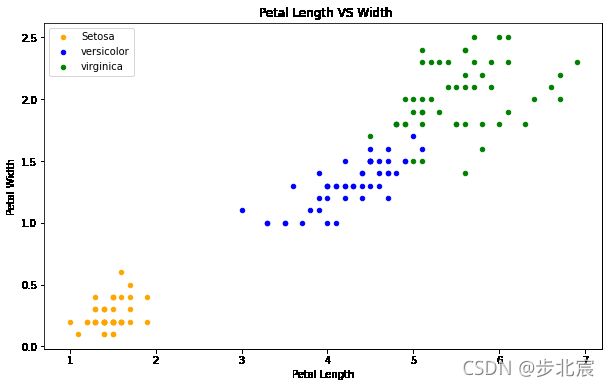
正如我们所看到的，与萼片特征相比，花瓣特征给出了更好的簇划分。这表明花瓣有助于更好、更准确地预测萼片。我们稍后再检查。

长度和宽度是如何分布的

iris.hist(edgecolor='black', linewidth=1.2)
fig=plt.gcf()
fig.set_size_inches(12,6)
plt.show()

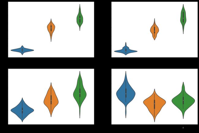
长度和宽度如何随物种而变化

seaborn.vinlinplot–绘制小提琴图

小提琴图是 箱型图 和核密度图的结合

展示了数据随种类的长度和密度。越窄的部分说明数据密度较低，越宽的部分说明数据密度高

plt.figure(figsize=(15,10))
plt.subplot(2,2,1)
sns.violinplot(x='Species',y='PetalLengthCm',data=iris)
plt.subplot(2,2,2)
sns.violinplot(x='Species',y='PetalWidthCm',data=iris)
plt.subplot(2,2,3)
sns.violinplot(x='Species',y='SepalLengthCm',data=iris)
plt.subplot(2,2,4)
sns.violinplot(x='Species',y='SepalWidthCm',data=iris)

分类算法

sklearn.linear_model —逻辑回归算法

sklearn.model_selection.train_test_split --将数据集随机分成训练集合测试集

sklearn.neighbors.KNeighborsClassifier --K临近算法

sklearn.svm --支持向量机算法

sklearn.metrics.accuracy——score --检查模型的准确性

sklearn.tree.DecisionTreeClassifier --决策树算法

from sklearn.linear_model import LogisticRegression
from sklearn.model_selection import train_test_split 
from sklearn.neighbors import KNeighborsClassifier 
from sklearn import svm  
from sklearn import metrics 
from sklearn.tree import DecisionTreeClassifier 

pandas.DataFrame.shape–返回DataFrame数据形状

iris.shape

(150, 5)

现在，当我们训练任何算法时，特征的数量及其相关性起着重要的作用。如果存在特征且许多特征高度相关，则训练具有所有特征的算法将降低精度。因此，应仔细选择特征。该数据集的功能较少，但我们仍将看到相关性。

pandas.DataFrame.corr–计算相关系数

seaborn.heatmap --热力图

plt.figure(figsize=(7,4)) 
sns.heatmap(iris.corr(),annot=True,cmap='cubehelix_r')
plt.show()

观察

萼片宽度和长度不相关，花瓣宽度和长度高度相关

我们将使用所有功能来训练算法并检查其准确性。然后我们将使用1个花瓣特征和1个萼片特征来检查算法的准确性，因为我们只使用2个不相关的特征。因此，我们可以在数据集中有一个方差，这可能有助于提高准确性。我们稍后再查。

训练算法步骤

1.将数据集拆分为培训和测试数据集。测试数据集通常比训练数据集小，因为它有助于更好地训练模型。

2.根据问题（分类或回归）选择算法。

3.然后将训练数据集传递给算法进行训练。我们使用.fit（）方法

4.然后将测试数据传递给经过训练的算法，以预测结果。我们使用.predict（）方法。

5.比较预测结果和真实值，给出算法准确性。

将数据拆分为训练和测试数据集

test_size = 0.3测试集数据占比30%

train, test = train_test_split(iris, test_size = 0.3)
print(train.shape)
print(test.shape)

(105, 5)
(45, 5)

获取训练集X的特征： [‘SepalLengthCm’,‘SepalWidthCm’,‘PetalLengthCm’,‘PetalWidthCm’]

训练集Y的实际分布

测试集X的特征

测试集Y的实际分布

train_X = train[['SepalLengthCm','SepalWidthCm','PetalLengthCm','PetalWidthCm']]
train_y=train.Species# output of our training data
test_X= test[['SepalLengthCm','SepalWidthCm','PetalLengthCm','PetalWidthCm']]
test_y =test.Species

检查训练集和测试集

train_X.head(2)

	SepalLengthCm	SepalWidthCm	PetalLengthCm	PetalWidthCm
72	6.3	2.5	4.9	1.5
39	5.1	3.4	1.5	0.2

test_X.head(2)

	SepalLengthCm	SepalWidthCm	PetalLengthCm	PetalWidthCm
143	6.8	3.2	5.9	2.3
40	5.0	3.5	1.3	0.3

训练集中分类的输出值（原始列表中标注的分类）

train_y.head()

72     1
39     0
21     0
109    2
106    2
Name: Species, dtype: int64

SVM支持向量机

sklearn.svm.SVC --SVC算法

sklearn.svm.SVC.fit–对于训练集使用fit方法训练算法

sklearn.svm.SVC.predict-- 传入测试集，使用predict方法给出预测值

sklearn.metrics.accuracy_score --预测值与实际值对比，给出算法准确度

model = svm.SVC()
model.fit(train_X,train_y) 
prediction=model.predict(test_X)
print('The accuracy of the SVM is:',metrics.accuracy_score(prediction,test_y))

The accuracy of the SVM is: 0.9777777777777777

支持向量机具有很好的精度。我们将继续检查不同型号的精度。现在我们将按照上面相同的步骤来训练各种机器学习算法。

逻辑回归（Logistic Regression）

model = LogisticRegression()
model.fit(train_X,train_y)
prediction=model.predict(test_X)
print('The accuracy of the Logistic Regression is',metrics.accuracy_score(prediction,test_y))

The accuracy of the Logistic Regression is 0.9777777777777777


D:\Anaconda3\lib\site-packages\sklearn\linear_model\_logistic.py:763: ConvergenceWarning: lbfgs failed to converge (status=1):
STOP: TOTAL NO. of ITERATIONS REACHED LIMIT.

Increase the number of iterations (max_iter) or scale the data as shown in:
    https://scikit-learn.org/stable/modules/preprocessing.html
Please also refer to the documentation for alternative solver options:
    https://scikit-learn.org/stable/modules/linear_model.html#logistic-regression
  n_iter_i = _check_optimize_result(

决策树（Decision Tree）

model=DecisionTreeClassifier()
model.fit(train_X,train_y)
prediction=model.predict(test_X)
print('The accuracy of the Decision Tree is',metrics.accuracy_score(prediction,test_y))

The accuracy of the Decision Tree is 0.9777777777777777

K均值聚类（Kmeans）

from  sklearn.cluster import KMeans

model = KMeans(n_clusters=3)
model.fit(train_X,train_y)
prediction=model.predict(test_X)
print('The accuracy of the KMeans is',metrics.accuracy_score(prediction,test_y))

x0 = (train_X,train_y)[prediction == 0]
x1 = (train_X,train_y)[prediction == 1]
x2 = (train_X,train_y)[prediction == 2]
plt.scatter(x0[:, 0], x0[:, 1], c = "red", marker='o', label='label0')  
plt.scatter(x1[:, 0], x1[:, 1], c = "green", marker='*', label='label1')  
plt.scatter(x2[:, 0], x2[:, 1], c = "blue", marker='+', label='label2')  
plt.xlabel('petal length')  
plt.ylabel('petal width')  
plt.legend(loc=2)  
plt.show()  

The accuracy of the KMeans is 0.3111111111111111



---------------------------------------------------------------------------

TypeError                                 Traceback (most recent call last)

 in 
      4 print('The accuracy of the KMeans is',metrics.accuracy_score(prediction,test_y))
      5 
----> 6 x0 = (train_X,train_y)[prediction == 0]
      7 x1 = (train_X,train_y)[prediction == 1]
      8 x2 = (train_X,train_y)[prediction == 2]


TypeError: only integer scalar arrays can be converted to a scalar index

K邻近算法（K-Nearest Neighbours）

n_neighbors=3：检查邻近3个点判断属于哪个分类

model=KNeighborsClassifier(n_neighbors=3) 
model.fit(train_X,train_y)
prediction=model.predict(test_X)
print('The accuracy of the KNN is',metrics.accuracy_score(prediction,test_y))

The accuracy of the KNN is 0.9777777777777777

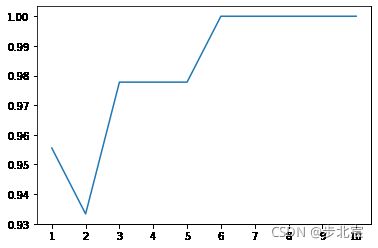
当n_neighbors值不同时，检查KNN算法的准确度变化，少数服从多数

a_index=list(range(1,11))
a=pd.Series()
x=[1,2,3,4,5,6,7,8,9,10]
for i in list(range(1,11)):
    model=KNeighborsClassifier(n_neighbors=i) 
    model.fit(train_X,train_y)
    prediction=model.predict(test_X)
    a=a.append(pd.Series(metrics.accuracy_score(prediction,test_y)))
plt.plot(a_index, a)
plt.xticks(x)

:2: DeprecationWarning: The default dtype for empty Series will be 'object' instead of 'float64' in a future version. Specify a dtype explicitly to silence this warning.
  a=pd.Series()





([,
  ,
  ,
  ,
  ,
  ,
  ,
  ,
  ,
  ],
 [Text(0, 0, ''),
  Text(0, 0, ''),
  Text(0, 0, ''),
  Text(0, 0, ''),
  Text(0, 0, ''),
  Text(0, 0, ''),
  Text(0, 0, ''),
  Text(0, 0, ''),
  Text(0, 0, ''),
  Text(0, 0, '')])

我们在上述模型中使用了iris的所有特征。现在我们将分别使用花瓣和萼片

创建花瓣和萼片训练数据

花萼：长度和宽度相关性很低

花瓣：长度和宽度相关性很高

petal=iris[['PetalLengthCm','PetalWidthCm','Species']]
sepal=iris[['SepalLengthCm','SepalWidthCm','Species']]

train_p,test_p=train_test_split(petal,test_size=0.3,random_state=0)  #petals
train_x_p=train_p[['PetalWidthCm','PetalLengthCm']]
train_y_p=train_p.Species
test_x_p=test_p[['PetalWidthCm','PetalLengthCm']]
test_y_p=test_p.Species


train_s,test_s=train_test_split(sepal,test_size=0.3,random_state=0)  #Sepal
train_x_s=train_s[['SepalWidthCm','SepalLengthCm']]
train_y_s=train_s.Species
test_x_s=test_s[['SepalWidthCm','SepalLengthCm']]
test_y_s=test_s.Species

SVM

model=svm.SVC()
model.fit(train_x_p,train_y_p) 
prediction=model.predict(test_x_p) 
print('The accuracy of the SVM using Petals is:',metrics.accuracy_score(prediction,test_y_p))

model=svm.SVC()
model.fit(train_x_s,train_y_s) 
prediction=model.predict(test_x_s) 
print('The accuracy of the SVM using Sepal is:',metrics.accuracy_score(prediction,test_y_s))

The accuracy of the SVM using Petals is: 0.9777777777777777
The accuracy of the SVM using Sepal is: 0.8

逻辑回归

model = LogisticRegression()
model.fit(train_x_p,train_y_p) 
prediction=model.predict(test_x_p) 
print('The accuracy of the Logistic Regression using Petals is:',metrics.accuracy_score(prediction,test_y_p))

model.fit(train_x_s,train_y_s) 
prediction=model.predict(test_x_s) 
print('The accuracy of the Logistic Regression using Sepals is:',metrics.accuracy_score(prediction,test_y_s))

The accuracy of the Logistic Regression using Petals is: 0.9777777777777777
The accuracy of the Logistic Regression using Sepals is: 0.8222222222222222

决策树

model=DecisionTreeClassifier()
model.fit(train_x_p,train_y_p) 
prediction=model.predict(test_x_p) 
print('The accuracy of the Decision Tree using Petals is:',metrics.accuracy_score(prediction,test_y_p))

model.fit(train_x_s,train_y_s) 
prediction=model.predict(test_x_s) 
print('The accuracy of the Decision Tree using Sepals is:',metrics.accuracy_score(prediction,test_y_s))

The accuracy of the Decision Tree using Petals is: 0.9555555555555556
The accuracy of the Decision Tree using Sepals is: 0.6444444444444445

K均值聚类

model=KMeans(n_clusters=3)
model.fit(train_x_p,train_y_p) 
prediction=model.predict(test_x_p) 
print('The accuracy of the KMeans using Petals is:',metrics.accuracy_score(prediction,test_y_p))

model.fit(train_x_s,train_y_s) 
prediction=model.predict(test_x_s) 
print('The accuracy of the KMeans using Sepals is:',metrics.accuracy_score(prediction,test_y_s))

The accuracy of the KMeans using Petals is: 0.022222222222222223
The accuracy of the KMeans using Sepals is: 0.7555555555555555

KNN

model=KNeighborsClassifier(n_neighbors=3) 
model.fit(train_x_p,train_y_p) 
prediction=model.predict(test_x_p) 
print('The accuracy of the KNN using Petals is:',metrics.accuracy_score(prediction,test_y_p))

model.fit(train_x_s,train_y_s) 
prediction=model.predict(test_x_s) 
print('The accuracy of the KNN using Sepals is:',metrics.accuracy_score(prediction,test_y_s))

The accuracy of the KNN using Petals is: 0.9777777777777777
The accuracy of the KNN using Sepals is: 0.7333333333333333

总结

使用花瓣覆盖萼片来训练数据可以提供更好的准确性。

正如我们在上面的热图中看到的，这是意料之中的，萼片宽度和长度之间的相关性非常低，而花瓣宽度和长度之间的相关性非常高。

结语

因此，我们刚刚实现了一些常见的机器学习算法。由于数据集很小，功能很少，所以我没有介绍一些概念，因为当我们有很多特征时，它们是相关的。