CVPR2022 A ConvNet for the 2020s
A ConvNet for the 2020s
https://arxiv.org/abs/2201.03545
https://github.com/facebookresearch/ConvNeXt
讲解https://mp.weixin.qq.com/s/q-s_dV4-TCiVPMOTZKEgPQ
https://www.bilibili.com/video/BV1SS4y157fu
https://www.bilibili.com/video/BV1iP4y1M7nk

以SwinTransformer的思路,在ResNet50和200上进行改造,优化
这篇文章的调参思路值得好好学习
Introduction
VIT在视觉领域比较火热,成为图像分类里的SOTA。缺点有,常规的VIT在解决像素密集的分类任务比如目标检测和语义分割,比较难。swin Transformer重新引入了几种ConvNet先验信息,让transformer性能更好。但这些都归功于transformer的内在优越性,而非卷积固有归纳偏置。
精度87.8%
本文使用现代的训练策略和超参数重新训练了ResNet50,发现提升了两个多点。这说明:Transformer与ConvNet的性能差距很大比例源自训练技术的升级。

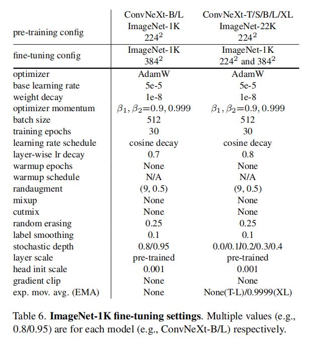
微调设置
Method
Macro Design

按照SwinTransformer中block的1131比例,将resnet50中3463调整为3393,准确率从78.8% 到 79.4%

然后把conv1(是将输入图像进行4倍下采样)替换为4*4卷积,stride为4,模仿VIT块化改造。
ResNeXt
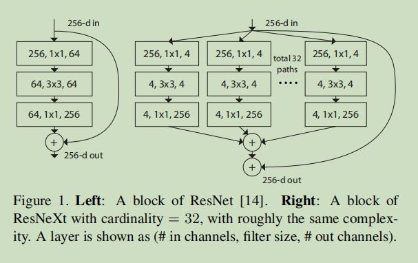
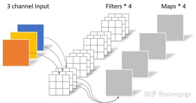
引入组卷积和深度可分离卷积,并将channel通道从64提升到96(也就是将network width提升),计算量大幅下降,准确率提升

Inverted Bottleneck
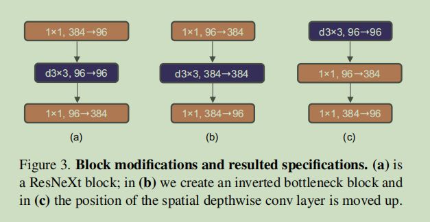
模仿MLP,把中间维度变成384,输入输出变成96
Large Kernel Size
将深度可分离卷积往前移动(Figure3 c),卷积核选择77最合适

Various Layer-wise Micro Design
概述一下结构,先是7x7的深度可分离组卷积(num_groups = in_channels),经过LN归一化层之后是两个1x1卷积来改变通道,在swin中就是两个MLP。11卷积其实就是在通道上的MLP

ReLU可以替换为ViT的GELU
更少的激活函数
移除两个BN层仅保留 1X1卷积之前的一个BN
BN换为LN
使用单独的下采样层
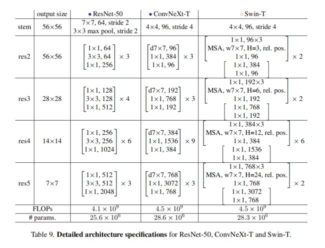
ResNet ConvNeXt Swin-T
代码学习
https://www.bilibili.com/video/BV11Y41137VA/

models/convnext.py核心代码
class Block(nn.Module):
    r""" ConvNeXt Block. There are two equivalent implementations:
    (1) DwConv -> LayerNorm (channels_first) -> 1x1 Conv -> GELU -> 1x1 Conv; all in (N, C, H, W)
    (2) DwConv -> Permute to (N, H, W, C); LayerNorm (channels_last) -> Linear -> GELU -> Linear; Permute back
    We use (2) as we find it slightly faster in PyTorch

    Args:
        dim (int): Number of input channels.
        drop_path (float): Stochastic depth rate. Default: 0.0
        layer_scale_init_value (float): Init value for Layer Scale. Default: 1e-6.
    """
    def __init__(self, dim, drop_path=0., layer_scale_init_value=1e-6):
        super().__init__()
        self.dwconv = nn.Conv2d(dim, dim, kernel_size=7, padding=3, groups=dim)
        # depthwise conv 前两个dim分别是输入和输出,
        # 组卷积的groups等于输入的dim
        self.norm = LayerNorm(dim, eps=1e-6)
        # LN层归一化,会先算出一个均值和方差,大小就是batch*H*W*通道数,归一化到正态分布
        #再引入权重和偏置,把张量变换到一个新的分布上
        self.pwconv1 = nn.Linear(dim, 4 * dim)
        # pointwise/1x1 convs,
        # implemented with linear layers,用Linear实现11 卷积,也可以用nn.conv2d
        # 放大到4倍的dim,384
        self.act = nn.GELU() # 激活函数
        self.pwconv2 = nn.Linear(4 * dim, dim)
        # 再映射回原来的dim也就是96
        self.gamma = nn.Parameter(layer_scale_init_value * torch.ones((dim)),
                                    requires_grad=True) if layer_scale_init_value > 0 else None
        self.drop_path = DropPath(drop_path) if drop_path > 0. else nn.Identity()

    def forward(self, x):
        input = x
        x = self.dwconv(x)
        x = x.permute(0, 2, 3, 1)
        # (N, C, H, W) -> (N, H, W, C)
        # permute是转置函数可以操作多个维度
        # 另一个转置函数transpose一次性操作只能两个维度
        x = self.norm(x)
        x = self.pwconv1(x)
        x = self.act(x)
        x = self.pwconv2(x)
        if self.gamma is not None:
            x = self.gamma * x
        x = x.permute(0, 3, 1, 2) # (N, H, W, C) -> (N, C, H, W)

        x = input + self.drop_path(x) # 残差连接
        return x
class ConvNeXt(nn.Module):
    r""" ConvNeXt
        A PyTorch impl of : `A ConvNet for the 2020s`  -
          https://arxiv.org/pdf/2201.03545.pdf

    Args:
        in_chans (int): Number of input image channels. Default: 3
        num_classes (int): Number of classes for classification head. Default: 1000
        depths (tuple(int)): Number of blocks at each stage. Default: [3, 3, 9, 3]
        dims (int): Feature dimension at each stage. Default: [96, 192, 384, 768]
        drop_path_rate (float): Stochastic depth rate. Default: 0.
        layer_scale_init_value (float): Init value for Layer Scale. Default: 1e-6.
        head_init_scale (float): Init scaling value for classifier weights and biases. Default: 1.
    """

    def __init__(self, in_chans=3, num_classes=1000,
                 depths=[3, 3, 9, 3], dims=[96, 192, 384, 768], drop_path_rate=0.,
                 # 把depth和dim用list存起来,depth是每个block的数量
                 layer_scale_init_value=1e-6, head_init_scale=1.,
                 ):
        super().__init__()

        self.downsample_layers = nn.ModuleList()  # stem and 3 intermediate downsampling conv layers
        stem = nn.Sequential(
            nn.Conv2d(in_chans, dims[0], kernel_size=4, stride=4),  # stem模块 ,输入为3,输出96,4*4卷积作为下采样
            LayerNorm(dims[0], eps=1e-6, data_format="channels_first")
        )
        self.downsample_layers.append(stem)  # 把stem放到更大的ModuleList容器中
        for i in range(3):  # 这是每个stage之后的空间下采样层,一共3个,用2*2卷积实现。每层前有一个LN。
            downsample_layer = nn.Sequential(
                LayerNorm(dims[i], eps=1e-6, data_format="channels_first"),
                nn.Conv2d(dims[i], dims[i + 1], kernel_size=2, stride=2),  # 输入是上一个stage的通道,输出是下一个stage的
            )
            self.downsample_layers.append(downsample_layer)

        self.stages = nn.ModuleList() # 4 feature resolution stages, each consisting of multiple residual blocks
        dp_rates=[x.item() for x in torch.linspace(0, drop_path_rate, sum(depths))]
        # linsapce 返回一个等差数列1维张量,包含在区间start和end上均匀间隔的step个点,drop_path_rate随机深度 ,返回sum(depths)个点
        # 网络越到后面dropout的比例更大
        cur = 0
        for i in range(4):
            stage = nn.Sequential(
                *[Block(dim=dims[i], drop_path=dp_rates[cur + j],
                layer_scale_init_value=layer_scale_init_value) for j in range(depths[i])]
            )
            self.stages.append(stage)
            cur += depths[i]

        self.norm = nn.LayerNorm(dims[-1], eps=1e-6) # final norm layer
        self.head = nn.Linear(dims[-1], num_classes) # 线性层,用来分类

        self.apply(self._init_weights)
        self.head.weight.data.mul_(head_init_scale)
        self.head.bias.data.mul_(head_init_scale)

    def _init_weights(self, m):
        if isinstance(m, (nn.Conv2d, nn.Linear)):
            trunc_normal_(m.weight, std=.02)
            nn.init.constant_(m.bias, 0)

    def forward_features(self, x):
        for i in range(4):
            x = self.downsample_layers[i](x) #每个stage之前的下采样
            x = self.stages[i](x)
        return self.norm(x.mean([-2, -1])) # global average pooling, (N, C, H, W) -> (N, C)  对-2,-1维度做平均池化,将向量变成N,C

    def forward(self, x):
        x = self.forward_features(x) # 把提取特征和后面的任务分离
        x = self.head(x)
        return x