天猫用户重复购买预测之数据分析

赛题理解

赛题链接
赛题背景：
商家有时会在特定日期，例如Boxing-day，黑色星期五或是双十一（11月11日）开展大型促销活动或者发放优惠券以吸引消费者，然而很多被吸引来的买家都是一次性消费者，这些促销活动可能对销售业绩的增长并没有长远帮助，因此为解决这个问题，商家需要识别出哪类消费者可以转化为重复购买者。通过对这些潜在的忠诚客户进行定位，商家可以大大降低促销成本，提高投资回报率（Return on Investment, ROI）。众所周知的是，在线投放广告时精准定位客户是件比较难的事情，尤其是针对新消费者的定位。不过，利用天猫长期积累的用户行为日志，我们或许可以解决这个问题。
我们提供了一些商家信息，以及在“双十一”期间购买了对应产品的新消费者信息。你的任务是预测给定的商家中，哪些新消费者在未来会成为忠实客户，即需要预测这些新消费者在6个月内再次购买的概率。
数据说明：
数据集主要包括在”双十一“之前和之后的六个月内，匿名用户购买的行为日志数据，用户的画像数据，以及相关的指示标签，标明其是否为重复购买用户。

• 用户行为日志

字段名称	描述
user_id	购物者的唯一ID编码
item_id	购物者的唯一ID编码
cat_id	商品所属品类的唯一编码
merchant_id	商家的唯一ID编码
brand_id	商品品牌的唯一编码
time_tamp	购买时间（格式：mmdd）
action_type	包含{0, 1, 2, 3}，0表示单击，1表示添加到购物车，2表示购买，3表示添加到收藏夹

• 用户画像

字段名称	描述
user_id	购物者的唯一ID编码
age_range	用户年龄范围。<18岁为1；[18,24]为2； [25,29]为3； [30,34]为4；[35,39]为5；[40,49]为6； > = 50时为7和8; 0和NULL表示未知
gender	用户性别。0表示女性，1表示男性，2和NULL表示未知

• 训练数据和测试数据

字段名称	描述
user_id	购物者的唯一ID编码
merchant_id	商家的唯一ID编码
label	包含{0, 1}，1表示重复买家，0表示非重复买家。测试集这一部分需要预测，因此为空。

评价指标：
$$AUC=\frac{{\sum }_{i\in positiveClass}ran{k}_i-\frac{M(1+M)}{2}}{M\ast N}$$
其中，M表示正样本个数，N表示负样本个数，AUC反映了模型对正负样本排序能力的强弱，对Score的大小和精度没有要求。
解题思路：

EDA

import pandas as pd
import numpy as np
import matplotlib.pyplot as plt
import seaborn as sns
import time
import scipy
import gc
from collections import Counter
import warnings
from matplotlib import rcParams

config = {
    "font.family":'Times New Roman',  # 设置字体类型
}

rcParams.update(config)
warnings.filterwarnings(action="ignore")

%matplotlib inline

# 数据存储情况
!tree data/data_format1/

[01;34mdata/data_format1/[00m
├── test_format1.csv
├── train_format1.csv
├── user_info_format1.csv
└── user_log_format1.csv

0 directories, 4 files

# 问题：如何优化读入数据的内存占用情况？

# 解释内存
def reduce_mem(df):
    """对于数值类型的数据进行内存节省"""
    
    starttime = time.time()
    numerics = ['int16', 'int32', 'int64', 'float16', 'float32', 'float64']
    start_mem = df.memory_usage().sum() / 1024**2  # 统计内存使用情况
    
    for col in df.columns:
        col_type = df[col].dtypes
        if col_type in numerics:
            c_min = df[col].min()
            c_max = df[col].max()
            if pd.isnull(c_min) or pd.isnull(c_max):
                continue
            if str(col_type)[:3] == 'int':
                # 装换数据类型
                if c_min > np.iinfo(np.int8).min and c_max < np.iinfo(np.int8).max:
                    df[col] = df[col].astype(np.int8)
                elif c_min > np.iinfo(np.int16).min and c_max < np.iinfo(np.int16).max:
                    df[col] = df[col].astype(np.int16)
                elif c_min > np.iinfo(np.int32).min and c_max < np.iinfo(np.int32).max:
                    df[col] = df[col].astype(np.int32)
                elif c_min > np.iinfo(np.int64).min and c_max < np.iinfo(np.int64).max:
                    df[col] = df[col].astype(np.int64)
            else:
                if c_min > np.finfo(np.float16).min and c_max < np.finfo(np.float16).max:
                    df[col] = df[col].astype(np.float16)
                elif c_min > np.finfo(np.float32).min and c_max < np.finfo(np.float32).max:
                    df[col] = df[col].astype(np.float32)
                else:
                    df[col] = df[col].astype(np.float64)
                    
    end_mem = df.memory_usage().sum() / 1024**2
    print('-- Mem. usage decreased to {:5.2f} Mb ({:.1f}% reduction),time spend:{:2.2f} min'.format(end_mem,
                                                                                                           100*(start_mem-end_mem)/start_mem,
                                                                                                           (time.time()-starttime)/60))
    return df

训练集

train_data = reduce_mem(pd.read_csv("./data/data_format1/train_format1.csv"))
train_data

-- Mem. usage decreased to  1.74 Mb (70.8% reduction),time spend:0.00 min

	user_id	merchant_id	label
0	34176	3906	0
1	34176	121	0
2	34176	4356	1
3	34176	2217	0
4	230784	4818	0
...	...	...	...
260859	359807	4325	0
260860	294527	3971	0
260861	294527	152	0
260862	294527	2537	0
260863	229247	4140	0

260864 rows × 3 columns

train_data.info()

RangeIndex: 260864 entries, 0 to 260863
Data columns (total 3 columns):
 #   Column       Non-Null Count   Dtype
---  ------       --------------   -----
 0   user_id      260864 non-null  int32
 1   merchant_id  260864 non-null  int16
 2   label        260864 non-null  int8 
dtypes: int16(1), int32(1), int8(1)
memory usage: 1.7 MB

train_data.nunique()

user_id        212062
merchant_id      1993
label               2
dtype: int64

用户信息表

user_info = reduce_mem(pd.read_csv("./data/data_format1/user_info_format1.csv"))
user_info

-- Mem. usage decreased to  3.24 Mb (66.7% reduction),time spend:0.00 min

	user_id	age_range	gender
0	376517	6.0	1.0
1	234512	5.0	0.0
2	344532	5.0	0.0
3	186135	5.0	0.0
4	30230	5.0	0.0
...	...	...	...
424165	395814	3.0	1.0
424166	245950	0.0	1.0
424167	208016	NaN	NaN
424168	272535	6.0	1.0
424169	18031	3.0	1.0

424170 rows × 3 columns

user_info.info()

RangeIndex: 424170 entries, 0 to 424169
Data columns (total 3 columns):
 #   Column     Non-Null Count   Dtype  
---  ------     --------------   -----  
 0   user_id    424170 non-null  int32  
 1   age_range  421953 non-null  float16
 2   gender     417734 non-null  float16
dtypes: float16(2), int32(1)
memory usage: 3.2 MB

user_info.nunique()

user_id      424170
age_range         9
gender            3
dtype: int64

用户行为数据

# 问题：如何在pandas读取大批量的数据?

# 数据量过大，采用迭代方法
reader = pd.read_csv("./data/data_format1/user_log_format1.csv", iterator=True)
# try:
#     df = reader.get_chunk(100000)
# except StopIteration:
#     print("Iteration is stopped.")
loop = True
chunkSize = 100000
chunks = []

while loop:
    try:
        chunk = reader.get_chunk(chunkSize)
        chunks.append(chunk)
    except StopIteration:
        loop = False
        print("Iteration is stopped.")
        
df = pd.concat(chunks, ignore_index=True)

user_log = reduce_mem(df)
user_log

	user_id	item_id	cat_id	seller_id	brand_id	time_stamp	action_type
0	328862	323294	833	2882	2660.0	829	0
1	328862	844400	1271	2882	2660.0	829	0
2	328862	575153	1271	2882	2660.0	829	0
3	328862	996875	1271	2882	2660.0	829	0
4	328862	1086186	1271	1253	1049.0	829	0
...	...	...	...	...	...	...	...
54925325	208016	107662	898	1346	7996.0	1110	0
54925326	208016	1058313	898	1346	7996.0	1110	0
54925327	208016	449814	898	983	7996.0	1110	0
54925328	208016	634856	898	1346	7996.0	1110	0
54925329	208016	272094	898	1346	7996.0	1111	0

54925330 rows × 7 columns

user_log["user_id"].nunique()

424170

user_log.info()

RangeIndex: 54925330 entries, 0 to 54925329
Data columns (total 7 columns):
 #   Column       Dtype  
---  ------       -----  
 0   user_id      int32  
 1   item_id      int32  
 2   cat_id       int16  
 3   seller_id    int16  
 4   brand_id     float16
 5   time_stamp   int16  
 6   action_type  int8   
dtypes: float16(1), int16(3), int32(2), int8(1)
memory usage: 890.5 MB

测试集信息表

test_data = reduce_mem(pd.read_csv("./data/data_format1/test_format1.csv"))
test_data

-- Mem. usage decreased to  3.49 Mb (41.7% reduction),time spend:0.00 min

	user_id	merchant_id	prob
0	163968	4605	NaN
1	360576	1581	NaN
2	98688	1964	NaN
3	98688	3645	NaN
4	295296	3361	NaN
...	...	...	...
261472	228479	3111	NaN
261473	97919	2341	NaN
261474	97919	3971	NaN
261475	32639	3536	NaN
261476	32639	3319	NaN

261477 rows × 3 columns

test_data.info()

RangeIndex: 261477 entries, 0 to 261476
Data columns (total 3 columns):
 #   Column       Non-Null Count   Dtype  
---  ------       --------------   -----  
 0   user_id      261477 non-null  int32  
 1   merchant_id  261477 non-null  int16  
 2   prob         0 non-null       float64
dtypes: float64(1), int16(1), int32(1)
memory usage: 3.5 MB

缺失值

# user_log 用户日志表
Total = user_log.isnull().sum().sort_values(ascending=False)
percent = (user_log.isnull().sum()/user_log.isnull().count()).sort_values(ascending=False)*100
missing_data = pd.concat([Total, percent], axis=1, keys=["Total", "Percent"])
missing_data

	Total	Percent
brand_id	91015	0.165707
user_id	0	0.000000
item_id	0	0.000000
cat_id	0	0.000000
seller_id	0	0.000000
time_stamp	0	0.000000
action_type	0	0.000000

结论：用户日志表中的特征信息缺失比例较小，且只出现在品牌一栏中，可以删除。

# user_info 用户信息表
Total = user_info.isnull().sum().sort_values(ascending=False)
percent = (user_info.isnull().sum()/user_info.isnull().count()).sort_values(ascending=False)*100
missing_data = pd.concat([Total, percent], axis=1, keys=["Total", "Percent"])
missing_data

	Total	Percent
gender	6436	1.517316
age_range	2217	0.522668
user_id	0	0.000000

结论：用户信息表中，用户性别和年龄缺失，考虑此特征为类别特征，可以使用众数填补, 注意缺失值不止为NULL。

年龄缺失

# 年龄字段数据取值情况
user_info["age_range"].unique()

array([ 6.,  5.,  4.,  7.,  3.,  0.,  8.,  2., nan,  1.], dtype=float16)

# 年龄为零或为空为缺失值，缺失条目为95131条
user_info[(user_info["age_range"] == 0) | (user_info["age_range"].isna())].count()

user_id      95131
age_range    92914
gender       90664
dtype: int64

# 不同年龄段的缺失用户数量，不统计空值
user_info.groupby("age_range")[["user_id"]].count()

	user_id
age_range
0.0	92914
1.0	24
2.0	52871
3.0	111654
4.0	79991
5.0	40777
6.0	35464
7.0	6992
8.0	1266

### 性别缺失

# 查看性别取值范围
user_info["gender"].unique()

array([ 1.,  0.,  2., nan], dtype=float16)

# 统计性别缺失情况
user_info[(user_info["gender"].isna()) | (user_info["gender"] == 2)].count()

user_id      16862
age_range    14664
gender       10426
dtype: int64

统计用户只有一个缺失值

# 注:count只统计非Nan的值，因此在user_id的数量能够表示真实的缺失数量
user_info[(user_info["gender"].isna()) | (user_info["gender"] == 2) | (user_info["age_range"] == 0) | (user_info["age_range"].isna())].count()

user_id      106330
age_range    104113
gender        99894
dtype: int64

正负样本统计

label_gp = train_data.groupby("label")["user_id"].count()
label_gp

label
0    244912
1     15952
Name: user_id, dtype: int64

fig, ax = plt.subplots(1, 2, figsize=(12, 6))
train_data["label"].value_counts().plot(kind="pie"
                                        , ax=ax[0]
                                        , shadow=True
                                        , explode=[0, 0.1]
                                        , autopct="%1.1f%%"
                                       )

sns.countplot(x="label", data=train_data, ax=ax[1])

​

结论：样本极度不平衡，使用负采样或过采样技术调整数据不平衡的情况。
知识点: countplot

探索影响复购的各种因素

分析不同店铺与复购的关系

train_data_merchant = train_data.copy()
top5_idx = train_data_merchant.merchant_id.value_counts().head().index.tolist()
# 增加一列用于标记Top商户和非Top商户，便于统计其复购情况
train_data_merchant["Top5"] = train_data_merchant["merchant_id"].map(lambda x: 1 if x in top5_idx else 0)
train_data_merchant = train_data_merchant[train_data_merchant.Top5 == 1]

sns.countplot(x="merchant_id", hue="label", data=train_data_merchant)

结论：不同商铺复购情况大不相同，商铺复购率较低。

查看店铺的复购分布

merchant_repeat_buy = [rate for rate in train_data.groupby("merchant_id")["label"].mean() if rate <= 1 and rate >0]
plt.figure(figsize=(8, 4))

ax1 = plt.subplot(1, 2, 1)
sns.distplot(merchant_repeat_buy, fit=scipy.stats.norm)

ax2 = plt.subplot(1, 2, 2)
res = scipy.stats.probplot(merchant_repeat_buy, plot=plt)

​

结论：用户店铺复购率分布在0.15左右，用户复购率较低，且不同店铺具有不同的复购率。（数据分布属于右偏）

查看用户的复购分布

user_repeat_buy = [rate for rate in train_data.groupby("user_id")["label"].mean() if rate <= 1 and rate >0]

plt.figure(figsize=(8, 4))
ax1 = plt.subplot(1, 2, 1)
sns.distplot(user_repeat_buy, fit=scipy.stats.norm)

ax2 = plt.subplot(1, 2, 2)
res = scipy.stats.probplot(user_repeat_buy, plot=plt)

结论：近六个月的用户主要集中在一次购买为主，较少出现重复购买的情况。

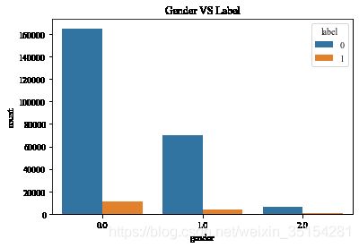
对用户性别的分析

train_data_user_info = train_data.merge(user_info, on=["user_id"], how="left")

plt.figure(figsize=(6, 4))
plt.title("Gender VS Label")
ax = sns.countplot(x="gender", hue="label", data=train_data_user_info)
for p in ax.patches:
    hight = p.get_height()

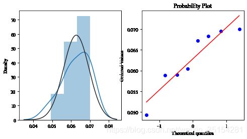
repeat_buy = [rate for rate in train_data_user_info.groupby("gender")["label"].mean() if rate <= 1 and rate >0]

plt.figure(figsize=(8, 4))
ax1 = plt.subplot(1, 2, 1)
sns.distplot(repeat_buy, fit=scipy.stats.norm)

ax2 = plt.subplot(1, 2, 2)
res = scipy.stats.probplot(repeat_buy, plot=plt)

结论：男女复购情况呈现差异性，女性购买情况远高于男性。

对用户年龄分析

plt.figure(figsize=(5, 4))
plt.title("Age VS Label")
res = sns.countplot(x="age_range", hue="label", data=train_data_user_info)

repeat_buy = [rate for rate in train_data_user_info.groupby("age_range")["label"].mean() if rate <= 1 and rate >0]

plt.figure(figsize=(8, 4))
ax1 = plt.subplot(1, 2, 1)
sns.distplot(repeat_buy, fit=scipy.stats.norm)

ax2 = plt.subplot(1, 2, 2)
res = scipy.stats.probplot(repeat_buy, plot=plt)

结论：用户在不同的年龄阶段复购情况有差异，年龄重点分布在25~34之间的用户。