数字图像处理第五章——图像复原与重建

目录

引言：

一、图像退化/复原过程的模型

二、噪声模型

2.1 噪声的空间与频率特性

2.2 一些重要的噪声高铝密度函数

2.2.1 高斯噪声

2.2.2 瑞利噪声

2.2.3 伽马噪声

2.2.4 指数噪声

2.2.5 均匀噪声

2.2.6 椒盐噪声（脉冲噪声）

2.2.7 python 实现

2.3 周期噪声

三、空间滤波

3.1 均值滤波器

3.1.1 算术均值滤波器

3.1.2 几何均值滤波器

3.1.3 谐波均值滤波器

3.1.4 逆谐波均值滤波器

3.1.5 python 实现

3.2 统计排序滤波器

3.2.1 中值滤波器

3.2.2 最大值和最小值滤波器

3.2.3 中点滤波器

3.2.4 修正的阿尔法均值滤波器

3.2.5 python实现

四、用频率域滤波消除周期噪声

4.1 带阻、带通滤波器

4.2 陷波滤波器

4.3 最佳陷波滤波器

五、线性位置不变的退化

六、逆滤波

七、最小均方误差（维纳）滤波

八、约束最小二乘方滤波、几何均值滤波

8.1 约束最小二乘方滤波

8.2 几何均值滤波 

---

引言：

        图像复原技术的主要目的是以预先确定的目标来改善图像，与图像增强不同的是，图像增强主要是一个主观过程，而图像复原则大部分是一个客观过程。图像复原试图利用退化现象的某种先验知识来复原被退化的图像。因而，复原技术是面向退化模型的，并且采用相反的过程进行处理，以便恢复出原图像。本章将从一幅退化数字图像的特点来考虑复原问题。

一、图像退化/复原过程的模型

        如图所示，退化过程可以被建模成一个退化函数和一个加性噪声项，对一幅输入图f(x,y)进行处理，在由退化函数与加性噪声的作用下生成一幅退化后的图像g(x,y)，后由复原滤波器进行复原最终得到一个原始图像的估计。在复原过程中，退化函数和加性噪声的信息知道的越多，最终得到的原始图像估计就会越接近f(x,y)。

        我们可以将空间域的退化图像用如下公式表示：

 将其放在频率域中时得到：

二、噪声模型

        数字图像中，噪声主要来源于图像的获取和/或传输过程。成像传感器的性能受到各种因素的影响，包括图像获取过程中的环境条件和传感器元器件自身的质量。

2.1 噪声的空间与频率特性

        噪声的空间特性主要是指定义噪声空间特性的参数以及噪声是否与图像相关，而频率特性则是指傅里叶域中噪声的频率内容，当噪声的傅里叶谱是常量时，噪声往往称为白噪声。除空间周期噪声外，在本章中我们假设噪声独立于空间坐标，并且噪声与图像本身不相关。

2.2 一些重要的噪声概率密度函数

2.2.1 高斯噪声

        在空间域和频率域中，由于高斯噪声在数学上的易处理性，故实践中常用这种噪声(也称为正态噪声)模型.事实上，这种易处理性非常方便，以至于高斯模型常常应用于在一定程度上导致最好结果的场所。

        高斯随机变量z的概率密度函数可由：

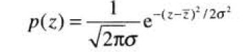
 其中，z为灰度值，表示z的均值，为z的标准差。

2.2.2 瑞利噪声

        瑞利噪声的概率密度函数为：

 其均值和方差分别为：

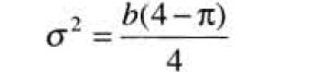
2.2.3 伽马噪声

        伽马噪声的概率密度函数为：

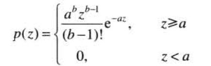
  其均值和方差分别为：

2.2.4 指数噪声

        指数噪声的概率密度函数为：

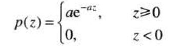
 其均值和方差分别为：

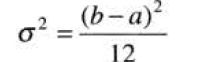
2.2.5 均匀噪声

        均匀噪声的概率密度函数为：

 其均值和方差分别为：

2.2.6 椒盐噪声（脉冲噪声）

        (双极)椒盐噪声的概率密度函数为：

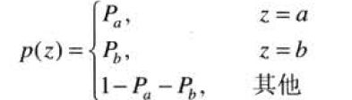
 若b>a，则灰度级b在图像中将显示为一个亮点，，反之，灰度级a在图像中将显示为一个暗点，若或为零，则脉冲噪声称为单极脉冲。如果和两者均不为零，尤其是两者近似相等时，脉冲噪声值将类似于在图像上随机分布的胡椒和盐粉微粒。

图为重要噪声概率密度波形

2.2.7 python 实现

import numpy as np
from matplotlib import pyplot as plt
import cv2
import random

img = cv2.imread('D:\\picture\\tupian.jpg')


# 量化
def normalize(image):
    return (image - image.min()) / (image.max() - image.min())

# 瑞利噪声
def ruili_noise(image, a):
    image = np.array(image, dtype=float)
    noise = np.random.rayleigh(a, size=image.shape)
    result = image + noise
    result = np.uint8(normalize(result) * 255)
    return result

# 伽马噪声
def gama_noise(image,scale):
    image = np.array(image, dtype=float)
    noise = np.random.gamma(shape=1, scale=scale, size=image.shape)
    result = image+noise
    result = np.uint8(normalize(result) * 255)
    return result


# 高斯噪声
def gaosi_noise(image, mean=0, var=0.001):
    image = np.array(image/255,dtype=float)
    noise = np.random.normal(mean, var ** 0.5, image.shape)#正态分布
    result = image + noise
    if result.min() < 0:
        clip = -1
    else:
        clip = 0
    result = np.clip(result, clip, 1.0)
    result = np.uint8(result * 255)
    return result


# 椒盐噪声
def jiaoyan_noise(image, pera):
    result = np.zeros(image.shape,np.uint8)
    perb = 1 - pera
    for i in range(image.shape[0]):
        for j in range(image.shape[1]):
            rod = random.random()
            if rod < pera:
                result[i][j] = 0
            elif rod > perb:
                result[i][j] = 255
            else:
                result[i][j] = image[i][j]
    return result


result1 = gaosi_noise(img, mean=0, var=0.06)
result2 = jiaoyan_noise(img, pera=0.3)
result3 = ruili_noise(img, a=30)
result4 = gama_noise(img, scale=50)

titles = ['original', 'gaosi', 'jiaoyan', 'ruili','gama']
images = [img, result1, result2, result3, result4]

plt.figure(figsize=(100, 20))
for i in range(5):
    plt.subplot(1, 5, i+1)
    plt.imshow(images[i], 'gray')
    plt.title(titles[i])
    plt.xticks([]), plt.yticks([])
plt.show()

2.3 周期噪声

        一幅图像中的周期噪声是在图像获取期间由电力或机电干扰产生的。 一幅图像中的周期噪声是在图像获取期间由电力或机电干扰产生的。

参考第5章 Python 数字图像处理(DIP) - 图像复原与重建7 - 周期噪声 余弦噪声生成方法_jasneik的博客-CSDN博客_python添加周期噪声

def normalize(image):  # 量化
    return (image - image.min()) / (image.max() - image.min())


def add_sin_noise(image, scale=1, angle=0):
    height, width = image.shape[:2]  # 原始高度

    # 转变角度
    if int(angle / 90) % 2 == 0:
        rotate_angle = angle % 90
    else:
        rotate_angle = 90 - (angle % 90)
    rotate_radian = np.radians(rotate_angle)
    new_height = int(np.ceil(height * np.cos(rotate_radian) + width * np.sin(rotate_radian)))
    new_width = int(np.ceil(width * np.cos(rotate_radian) + height * np.sin(rotate_radian)))

    if new_height < height:
        new_height = height
    if new_width < width:
        new_width = width

    u = np.arange(new_width)
    v = np.arange(new_height)
    u, v = np.meshgrid(u, v)

    noise = 1 - np.sin(u * scale)

    C1 = cv2.getRotationMatrix2D((new_width / 2.0, new_height / 2.0), angle, 1)
    new_img = cv2.warpAffine(noise, C1, (int(new_width), int(new_height)), borderValue=0)

    offset_height = abs(new_height - height) // 2
    offset_width = abs(new_width - width) // 2
    img_dst = new_img[offset_height:offset_height + height, offset_width:offset_width + width]
    result = normalize(img_dst)

    return result


def spectrum_fft(fft):
    return np.sqrt(np.power(fft.real, 2) + np.power(fft.imag, 2))

image = cv2.imread('D:\\picture\\tupian.jpg',0)

noise = add_sin_noise(image, scale=0.35, angle=-20)
img = np.array(image / 255, np.float32)
result1 = img + noise
result1 = np.uint8(normalize(result1)*255)

# 频率域中的其他特性
# FFT
img_fft = np.fft.fft2(result1.astype(np.float32))
# 中心化
fshift = np.fft.fftshift(img_fft)            # 将变换的频率图像四角移动到中心
# 中心化后的频谱
spectrum_fshift = spectrum_fft(fshift)
spectrum_fshift_n = np.uint8(normalize(spectrum_fshift) * 255)

# 对频谱做对数变换
spectrum_log = np.log(1 + spectrum_fshift)

plt.figure(figsize=(15, 10))
plt.subplot(131), plt.imshow(image, 'gray'),plt.title('orginal'), plt.xticks([]), plt.yticks([])
plt.subplot(132), plt.imshow(result1, 'gray'), plt.title('With Sine noise'), plt.xticks([]), plt.yticks([])
plt.subplot(133), plt.imshow(spectrum_log, 'gray'), plt.title('Spectrum'), plt.xticks([]), plt.yticks([])
plt.show()

三、空间滤波

当一幅图像中唯一存在的退化是噪声时

空间域：

频率域：

        由于我们无法得知噪声项的数值，因此从退化函数中直接消去噪声信号是不现实的，在周期噪声的情况下，由G(u,v)的谱来估计N(u,v)通常是可能的。当仅存在加性噪声的情况下，可以选择空间滤波方法。

3.1 均值滤波器

3.1.1 算术均值滤波器

        最简单的均值滤波器，在定义的区域中计算被污染图像g(x,y)的平均值：

3.1.2 几何均值滤波器

        几何均值滤波器复原的图像可由如下表达式给出：

 相较于算术均值滤波器而言丢失的图像细节减少。

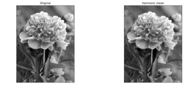
3.1.3 谐波均值滤波器

        谐波均值滤波器复原的图像可由如下表达式给出：

谐波均值滤波器适用于处理盐粒噪声，对于胡椒噪声的处理效果不是很好。

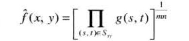
3.1.4 逆谐波均值滤波器

        逆谐波均值滤波器复原的图像可由如下表达式给出：

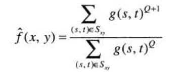
        其中Q称为滤波器的阶数.这种滤波器适合减少或在实际中消除椒盐噪声的影响.当Q值为正时，该滤波器消除胡椒噪声；当Q值为负时，该滤波器消除盐粒噪声.但它不能同时消除这两种噪声.注意，当Q=0时，逆谐波均值滤波器简化为算术均值滤波器；而当Q=-1时，则为谐波均值滤波器。

3.1.5 python 实现

算术均值滤波器

def arithmentic(image, kernel):

    img_h = image.shape[0]
    img_w = image.shape[1]

    m, n = kernel.shape[:2]

    pad_h = int((m - 1) / 2)
    pad_w = int((n - 1) / 2)

    image_pad = np.pad(image, ((pad_h, m - 1 - pad_h),
                               (pad_w, n - 1 - pad_w)), mode="edge")

    image_mean = image.copy()
    for i in range(pad_h, img_h + pad_h):
        for j in range(pad_w, img_w + pad_w):
            temp = np.sum(image_pad[i - pad_h:i + pad_h + 1, j - pad_w:j + pad_w + 1])
            image_mean[i - pad_h][j - pad_w] = 1 / (m * n) * temp
    return image_mean
img_ori = cv2.imread('D:\\picture\\tupian.jpg', 0)

mean_kernal = np.ones([3, 3])
mean_kernal = mean_kernal / mean_kernal.size

img_arithmentic = arithmentic(img_ori, kernel=mean_kernal)

img_cv2_mean = cv2.filter2D(img_ori, ddepth=-1, kernel=mean_kernal)

plt.figure(figsize=(18, 6))
plt.subplot(121), plt.imshow(img_ori, 'gray'), plt.title('original'), plt.xticks([]), plt.yticks([])
plt.subplot(122), plt.imshow(img_arithmentic, 'gray'), plt.title('math'), plt.xticks([]), plt.yticks([])
plt.show()

 几何均值滤波器

def geometric(image, kernel):
    img_h = image.shape[0]
    img_w = image.shape[1]

    m, n = kernel.shape[:2]
    order = 1 / (kernel.size)

    pad_h = int((m - 1) / 2)
    pad_w = int((n - 1) / 2)


    image_pad = np.pad(image.copy(), ((pad_h, m - 1 - pad_h),
                                      (pad_w, n - 1 - pad_w)), mode="edge")

    image_mean = image.copy()

    for i in range(pad_h, img_h + pad_h):
        for j in range(pad_w, img_w + pad_w):
            prod = np.prod(image_pad[i - pad_h:i + pad_h + 1, j - pad_w:j + pad_w + 1] * 1.0)
            image_mean[i - pad_h][j - pad_w] = np.power(prod, order)

    return image_mean

img = cv2.imread('D:\\picture\\tupian.jpg', 0)

kernal = np.ones([3, 3])
arithmetic_kernel = kernal / kernal.size

result = geometric(img, kernel=kernal)

plt.figure(figsize=(18, 6))
plt.subplot(121), plt.imshow(img, 'gray'), plt.title('Original'), plt.xticks([]), plt.yticks([])
plt.subplot(122), plt.imshow(result, 'gray'), plt.title('Geomentric Mean'), plt.xticks([]), plt.yticks([])
plt.show()

 谐波均值滤波器

def harmonic(image, kernel):
    e = 1e-8
    img_h = image.shape[0]
    img_w = image.shape[1]

    m, n = kernel.shape[:2]
    order = kernel.size

    pad_h = int((m - 1) / 2)
    pad_w = int((n - 1) / 2)

    image_pad = np.pad(image.copy(), ((pad_h, m - 1 - pad_h),
                                      (pad_w, n - 1 - pad_w)), mode="edge")

    image_mean = image.copy()
    for i in range(pad_h, img_h + pad_h):
        for j in range(pad_w, img_w + pad_w):
            temp = np.sum(
                1 / (image_pad[i - pad_h:i + pad_h + 1, j - pad_w:j + pad_w + 1] * 1.0 + e))
            image_mean[i - pad_h][j - pad_w] = order / temp

    return image_mean
img = cv2.imread('D:\\picture\\test.jpg', 0)

mean_kernal = np.ones([3, 3])
arithmetic_kernel = mean_kernal / mean_kernal.size

img_harmonic = harmonic(img, kernel=mean_kernal)

plt.figure(figsize=(18, 6))
plt.subplot(121), plt.imshow(img, 'gray'), plt.title('Original'), plt.xticks([]), plt.yticks([])
plt.subplot(122), plt.imshow(img_harmonic, 'gray'), plt.title('Harmonic mean'), plt.xticks([]), plt.yticks([])
plt.show()

 逆谐波均值滤波器

def iharmonic(image, kernel, Q=0):
    e = 1e-8
    img_h = image.shape[0]
    img_w = image.shape[1]

    m, n = kernel.shape[:2]

    pad_h = int((m - 1) / 2)
    pad_w = int((n - 1) / 2)

    image_pad = np.pad(image.copy(), ((pad_h, m - 1 - pad_h),
                                      (pad_w, n - 1 - pad_w)), mode="edge")

    image_mean = image.copy()
    for i in range(pad_h, img_h + pad_h):
        for j in range(pad_w, img_w + pad_w):
            temp = image_pad[i - pad_h:i + pad_h + 1, j - pad_w:j + pad_w + 1] * 1.0 + e
            image_mean[i - pad_h][j - pad_w] = np.sum(np.power(temp, (Q + 1))) / np.sum(
                np.power(temp, Q) + e)

    return image_mean
img_ori = cv2.imread('D:\\picture\\test.jpg', 0)

kernel = np.ones([3, 3])
arithmetic_kernel = kernel / kernel.size

img_iharmonic = iharmonic(img_ori, kernel=kernel, Q=1.5)

plt.figure(figsize=(18, 6))
plt.subplot(121), plt.imshow(img_ori, 'gray'), plt.title('Original'), plt.xticks([]), plt.yticks([])
plt.subplot(122), plt.imshow(img_iharmonic, 'gray'), plt.title('Iharmonic Mean'), plt.xticks([]), plt.yticks([])
plt.show()

3.2 统计排序滤波器

3.2.1 中值滤波器

        中值滤波器就像其名字所暗示的那样，使用一个像素邻域中的灰度级的中值来替代该像素的值：

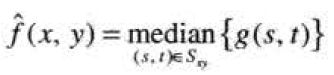
在(x,y)处的像素值是计算的中值.中值滤波器的应用非常普遍，因为对于某些类型的随机噪声，它们可提供良好的去噪能力，且比相同尺寸的线性平滑滤波器引起的模糊更少。

3.2.2 最大值和最小值滤波器

        统计学中的排列本身还有很多其他的可能性，可以使用序列中最后一个数值，称为最大值滤波器：

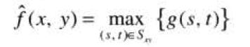
 这种滤波器对于发现图像中的最亮点非常有用.同样，因为胡椒噪声的值非常低，作为子图像区域 中这种最大值选择过程的结果，可以用这种滤波器降低它。

        选择起始值的滤波器被称为最小值滤波器：

 最小值滤波器对于发现图像中的最暗点非常有用，可以降低盐粒噪声。

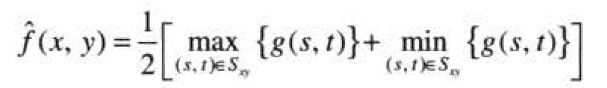
3.2.3 中点滤波器

        中点滤波器简单的计算滤波器包围区域中最大值和最小值之间的中点：

3.2.4 修正的阿尔法均值滤波器

        假设在邻域内去掉g(s,t)最低灰度值的d/2和最高灰度值的d/2，令代表剩下的mn-d个像素。由这些剩余像素的平均值形成的滤波器就叫做修正的阿尔法均值滤波器：

3.2.5 python实现

中值、最大值、最小值、中点、修正阿尔法滤波器

def median(image, kernel):  # 中值滤波器

    height, width = image.shape[:2]
    m, n = kernel.shape[:2]

    pad_h = int((m - 1) / 2)
    pad_w = int((n - 1) / 2)

    image_pad = np.pad(image, ((pad_h, m - 1 - pad_h),
                               (pad_w, n - 1 - pad_w)), mode="edge")

    image_result = np.zeros(image.shape)
    for i in range(height):
        for j in range(width):
            temp = image_pad[i:i + m, j:j + n]
            image_result[i, j] = np.median(temp)
    return image_result


def max(image, kernel):  # 最大值

    height, width = image.shape[:2]
    m, n = kernel.shape[:2]

    pad_h = int((m - 1) / 2)
    pad_w = int((n - 1) / 2)

    image_pad = np.pad(image, ((pad_h, m - 1 - pad_h),
                               (pad_w, n - 1 - pad_w)), mode="constant", constant_values=0)

    img_result = np.zeros(image.shape)
    for i in range(height):
        for j in range(width):
            temp = image_pad[i:i + m, j:j + n]
            img_result[i, j] = np.max(temp)
    return img_result


def min(image, kernel):  # 最小值

    height, width = image.shape[:2]
    m, n = kernel.shape[:2]

    pad_h = int((m - 1) / 2)
    pad_w = int((n - 1) / 2)

    image_pad = np.pad(image, ((pad_h, m - 1 - pad_h),
                               (pad_w, n - 1 - pad_w)), mode="edge")

    img_result = np.zeros(image.shape)
    for i in range(height):
        for j in range(width):
            temp = image_pad[i:i + m, j:j + n]
            img_result[i, j] = np.min(temp)
    return img_result


def middle(image, kernel):  # 中点

    height, width = image.shape[:2]
    m, n = kernel.shape[:2]

    pad_h = int((m - 1) / 2)
    pad_w = int((n - 1) / 2)

    image_pad = np.pad(image, ((pad_h, m - 1 - pad_h),
                               (pad_w, n - 1 - pad_w)), mode="edge")

    img_result = np.zeros(image.shape)
    for i in range(height):
        for j in range(width):
            temp = image_pad[i:i + m, j:j + n]
            img_result[i, j] = int(temp.max() / 2 + temp.min() / 2)
    return img_result


def modified_alpha(image, kernel, d=0):

    height, width = image.shape[:2]
    m, n = kernel.shape[:2]

    pad_h = int((m - 1) / 2)
    pad_w = int((n - 1) / 2)

    image_pad = np.pad(image, ((pad_h, m - 1 - pad_h),
                               (pad_w, n - 1 - pad_w)), mode="edge")

    img_result = np.zeros(image.shape)
    for i in range(height):
        for j in range(width):
            temp = np.sum(image_pad[i:i + m, j:j + n] * 1)
            img_result[i, j] = temp / (m * n - d)
    return img_result


img = cv2.imread('D:\\picture\\test.jpg', 0)

kernel = np.ones([3, 3])
img_median = median(img, kernel=kernel)
img_max = max(img, kernel=kernel)
img_min = min(img, kernel=kernel)
img_middle = middle(img, kernel=kernel)
img_modified = modified_alpha(img, kernel=kernel, d=1)
plt.figure(figsize=(15, 10))
image = [img_median, img_max, img_min, img_middle,img_modified]
name = ['median', 'max', 'min', 'middle', 'modified']

for i in range(5):
    plt.subplot(1, 5, i+1)
    plt.imshow(image[i], 'gray')
    plt.title(name[i])
    plt.xticks([]), plt.yticks([])
plt.show()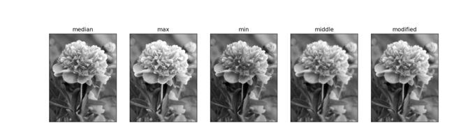

四、用频率域滤波消除周期噪声

4.1 带阻、带通滤波器

 从左往右分别为理想滤波器、布特沃斯滤波器、高斯带阻滤波器的透视图

        带阻滤波器的主要应用之一是在频率域噪声分量的一般位置近似已知的应用中消除噪声。一个典型的例子就是一幅被加性周期噪声污染的图像，该噪声可被近似为二维正弦函数.不难看出，一个正弦波的傅里叶变换由两个脉冲组成，它们是关于变换域坐标原点互为镜像的图像。

4.2 陷波滤波器

        陷波滤波器阻止(或通过)事先定义的中心频率的邻域内的频率。由于傅里叶变换的对称性，要获得有效的结果，陷波滤波器必须以关于原点对称的形式出现.这个原则的特例是，如果陷波滤波器位于原点处，在这种情况下，陷波滤波器是其本身。

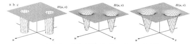
 从左往右分别为理想、布特沃斯、高斯陷波滤波器的透视图

 因为滤波器执行与陷阻滤波器完全相反的功能，所以传递函数为：

 是陷波滤波器的传递函数，这个陷波滤波器与传递函数为的陷波滤波器相对应 。

4.3 最佳陷波滤波器

        当同时存在多种干扰分量时，先前提及的滤波器就不再适用了，因为它们在进行滤波时可能会消除太多的图像信息。另外，干扰成分通常不是单频脉冲，相反，它们通常有携带干扰模式信息的宽边缘。从正常的变换背景中有时不容易检测到这些边缘。在许多应用中，降低这些退化影响时选择滤波方法将非常有用。

        该过程由两步组成，第-一步屏蔽干扰的主要成分，然后从被污染的图像中减去该模式的一个可变的加权部分.虽然我们是在一个特定的应用中来研究这一过程，但这个基本方法仍然十分通用，而且能应用到其他复原工作中，在这些复原工作中，多周期性干扰是主要问题。

        第一步提取主频率分量，如果滤波器构建只可通过与干扰模式相关的分量，那么干扰噪声的傅里叶变换由下式给出：

        G(u,v)为被污染图像的傅里叶变换。的形式需要多方面判断哪些是尖峰噪声干扰，为此，通常需要观察显示的G(u,v)的频谱来交互的创建陷波带通滤波器。空间下的相应模式可由：

        因为被污染的图像假设是由未污染的图像f(x,y)与干扰相加形成的，若完全已知，则从g(x,y)减去该干扰模式得到f(x,y)将是非常简单的事情。

 由此可以得到f(x,y)的估计值。估计值的局部方差可根据样本估计:

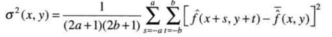
平均值为：

进一步我们可以得到：

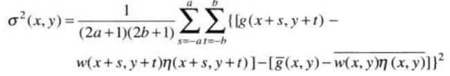
运算后得到：

五、线性位置不变的退化

        图像在复原前输入输出关系为：

 在线性系统H下，表示为：

 对于线性算子H其具有加性和均匀性的特点，当：

则算子称为位置不变系统，即图像的任意一点处的响应只取决于该点处的输入值，与位置无关。

对于离散冲激函数的定义，这里我们可以将其表示为：

假设=0：

H为线性算子：

使用均匀性：

而：

因此我们可以进一步得到：

在有加性噪声的情况下，线性退化模型的表达式可以变为：

在频域中就可以得到：

六、逆滤波

        研究退化函数H退化的图像复原的最初手段。利用退化函数除退化图像的傅里叶变换G(u,v)来计算原始图像傅里叶变换的估计。

由上面的内容我们得知：

代入，就可以得到

参考第5章 Python 数字图像处理(DIP) - 图像复原与重建14 - 逆滤波_jasneik的博客-CSDN博客_python逆滤波

中给出的python代码，在成功运行后，可以得到：

七、最小均方误差（维纳）滤波

维纳误差的公式为：

def motion_process(image_size, motion_angle, degree=15):

    PSF = np.zeros(image_size)
    center_position = (image_size[0] - 1) / 2
    slope_tan = math.tan(motion_angle * math.pi / 180)
    slope_cot = 1 / slope_tan
    if slope_tan <= 1:
        for i in range(degree):
            offset = round(i * slope_tan)
            PSF[int(center_position + offset), int(center_position - offset)] = 1
        return PSF / PSF.sum()
    else:
        for i in range(degree):
            offset = round(i * slope_cot)
            PSF[int(center_position - offset), int(center_position + offset)] = 1
        return PSF / PSF.sum()


def get_motion_dsf(image_size, motion_angle, motion_dis):

    PSF = np.zeros(image_size)
    x_center = (image_size[0] - 1) / 2
    y_center = (image_size[1] - 1) / 2

    sin_val = np.sin(motion_angle * np.pi / 180)
    cos_val = np.cos(motion_angle * np.pi / 180)

    for i in range(motion_dis):
        x_offset = round(sin_val * i)
        y_offset = round(cos_val * i)
        PSF[int(x_center - x_offset), int(y_center + y_offset)] = 1

    return PSF / PSF.sum()

def make_blurred(input, PSF, eps):

    input_fft = np.fft.fft2(input)
    PSF_fft = np.fft.fft2(PSF) + eps
    blurred = np.fft.ifft2(input_fft * PSF_fft)
    blurred = np.abs(np.fft.fftshift(blurred))
    return blurred


def wiener(input, PSF, eps, K=0.01):
    input_fft = np.fft.fft2(input)
    PSF_fft = np.fft.fft2(PSF) + eps
    PSF_fft_1 = np.conj(PSF_fft) / (np.abs(PSF_fft) ** 2 + K)
    result = np.fft.ifft2(input_fft * PSF_fft_1)
    result = np.abs(np.fft.fftshift(result))
    return result

if __name__ == "__main__":
    image = cv2.imread('D:\\picture\\test.jpg', 0)
    PSF = get_motion_dsf(image.shape[:2], -50, 100)
    blurred = make_blurred(image, PSF, 1e-3)
    plt.subplot(141), plt.imshow(blurred, 'gray'), plt.title("Motion blurred")
    plt.xticks([]), plt.yticks([])
    result = wiener(blurred, PSF, 1e-3)
    plt.subplot(142), plt.imshow(result, 'gray'), plt.title("wiener deblurred(k=0.01)")
    plt.xticks([]), plt.yticks([])
    blurred_noisy = blurred + 0.1 * blurred.std() * np.random.standard_normal(blurred.shape)
    plt.subplot(143), plt.imshow(blurred_noisy, 'gray'), plt.title("motion & noisy blurred")
    plt.xticks([]), plt.yticks([])
    result = wiener(blurred_noisy, PSF, 0.1 + 1e-3)
    plt.subplot(144), plt.imshow(result, 'gray'), plt.title("wiener deblurred(k=0.01)")
    plt.xticks([]), plt.yticks([])
    plt.tight_layout()
    plt.show()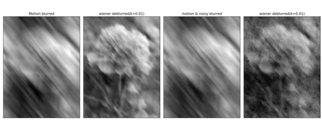

八、约束最小二乘方滤波、几何均值滤波

8.1 约束最小二乘方滤波

P(u,v)为：

8.2 几何均值滤波 

def puv(image):
    h, w = image.shape[:2]

    h_pad, w_pad = h - 3, w - 3
    p_xy = np.array([[0, -1, 0],
                     [-1, 4, -1],
                     [0, -1, 0]])
    p_pad = np.pad(p_xy, ((h_pad // 2, h_pad - h_pad // 2), (w_pad // 2, w_pad - w_pad // 2)), mode='constant')
    p_uv = np.fft.fft2(p_pad)
    return p_uv


def motion(image_size, motion_angle, motion_dis):

    PSF = np.zeros(image_size)
    x_center = (image_size[0] - 1) / 2
    y_center = (image_size[1] - 1) / 2

    sin_val = np.sin(motion_angle * np.pi / 180)
    cos_val = np.cos(motion_angle * np.pi / 180)

    for i in range(motion_dis):
        x_offset = round(sin_val * i)
        y_offset = round(cos_val * i)
        PSF[int(x_center - x_offset), int(y_center + y_offset)] = 1

    return PSF / PSF.sum()


def blurred(input, PSF, eps):

    input_fft = np.fft.fft2(input)
    PSF_fft = np.fft.fft2(PSF) + eps
    blurred = np.fft.ifft2(input_fft * PSF_fft)
    blurred = np.abs(np.fft.fftshift(blurred))
    return blurred


def geometric(image, PSF, eps, K=1, alpha=1, beta=1):
    fft = np.fft.fft2(image)
    PSF_fft = np.fft.fft2(PSF)
    conj = PSF_fft.conj()
    abs_square = (PSF_fft * conj).real
    huv = np.power(conj / (abs_square), alpha) * np.power(conj / (abs_square + beta*(K)), 1 - alpha)
    result = np.fft.ifft2(fft * huv)
    result = np.abs(np.fft.fftshift(result))
    return result


def square(image, PSF, eps, gamma=0.01):

    fft = np.fft.fft2(image)
    PSF_fft = np.fft.fft2(PSF)
    conj = PSF_fft.conj()
    p_uv = puv(image)
    abs_conj = np.abs(PSF_fft) ** 2
    huv = conj / (abs_conj + gamma * (np.abs(p_uv) ** 2))
    result = np.fft.ifft2(fft * huv)
    result = np.abs(np.fft.fftshift(result))
    return result, abs_conj


image = cv2.imread('D:\\picture\\test.jpg', 0)
PSF = motion(image.shape[:2], -50, 100)
blurred = blurred(image, PSF, 1e-5)

least_square, abs_con = square(blurred, PSF, 1e-5, gamma=1e-6)
least_square = np.uint8(normalize(least_square) * 255)

geometric_mean = geometric(blurred, PSF, 1e-5, K=1, alpha=1/2, beta=0)
geometric_mean = np.uint8(normalize(geometric_mean) * 255)

img_diff = image - least_square
plt.figure(figsize=(15, 5))
plt.subplot(141), plt.imshow(image,'gray'), plt.title("original"), plt.xticks([]), plt.yticks([])
plt.subplot(142), plt.imshow(blurred, 'gray'), plt.title("Motion blurred"), plt.xticks([]), plt.yticks([])
plt.subplot(143), plt.imshow(least_square, 'gray'), plt.title("Least Square Filter"), plt.xticks([]), plt.yticks([])
plt.subplot(144), plt.imshow(geometric_mean, 'gray'), plt.title("Geometric mean Filter"), plt.xticks([]), plt.yticks([])
plt.tight_layout()
plt.show()