【机器学习】LSTM 讲解

2. LSTM

2.1. 长期依赖问题

标准 RNN 结构在理论上完全可以实现将最初的信息保留到即使很远的时刻，但是在实践中发现 RNN 会受到短时记忆的影响。如果一条序列足够长，那它们将很难将信息从较早的时刻传送到后面的时刻。 因此，如果正在尝试处理一段文本进行预测，RNN 可能从一开始就会遗漏重要信息。比如我们尝试预测 “I grew up in France … I speak fluent French” 这句话的最后一个词 ”French“ 。当前的信息（“I speak fluent”）表明接下来的单词是很可能是语言的名字。但是需要哪种语言，我们就要根据离当前位置很远的 “France” 来确定。这就说明相关信息和当前预测词的位置之间的间隔可能非常大，随着这间隔不断变大，RNN 就会失去学习连接如此远的信息的能力。 这就是我们上面提到的 RNN 最致命的缺点。

为了解决这个问题，提出了 LSTM 。

2.2. 网络结构

LSTM 属于 RNN 的扩展模型，二者的区别仅在于每个单元内部结构不同。LSTM 单元结构如下。

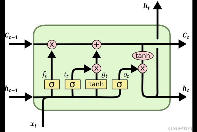
其中，黄色矩形表示一层神经网络，包含权重和激活函数，矩形中的符号表明激活函数的类型，$\sigma$ 对应 sigmoid 函数，$\tanh$ 对应 tanh 函数；粉色（椭）圆表示逐元素操作，比如粉色（椭）圆中为乘号表明矩阵进行对应元素相乘（点乘）操作，$\tanh$ 表明进行逐元素取 tanh 值。

下图展示了 LSTM 单元的完整前向传播过程。

从”遗忘门“、”输入门“和”输出门“，这三个”门“的角度来理解 LSTM 单元。

之所以称之为”门“，是考虑到生活中的”门“存在”开/闭“两种状态。LSTM 单元中的”门“也是存在”开/闭“两种状态，”开“表示全部（绝大部分）信息都可以经过”门“流出，”闭“表示全部（绝大部分）信息都不能经过”门“流出，而是被”门“过滤掉。由于 sigmoid 函数非常适合二分类，所以该函数在 LSTM 单元中起到”门“过滤的作用，用于控制信息是否流出（流出量）。

• 遗忘门

  ”遗忘门“决定了前一个单元的状态 $c_{t-1}$ 有多少信息保留到当前单元状态 $c_t$ 中。对应图中过程 $[h_{t-1},x_t]\to f_t$ 。

• 输入门

  ”输入门“决定了当前单元的输入 $x_t$ 有多少信息保存到单元状态 $c_t$ 。对应图中过程 $[h_{t-1},x_t]\to i_t$ 。

• 输出门

  ”输出门“用于控制当前单元的状态 $c_t$ 有多少信息输出到当前输出值 $h_t$ 。对应图中过程 $[h_{t-1},x_t]\to o_t$ 。​

模型单元的思想可以理解为，$[h_{t-1},x_t]$ 经过遗忘门确定保留多少前一个单元的信息，$c_{t-1}$ 和 $\sigma (W_{xf}{x}_t+W_{hf}{h}_{t-1}+b_f)$ 按位点乘实现筛选出要保留的信息；$\sigma (W_{xi}{x}_t+W_{hi}{h}_{t-1}+b_i)$ 和 $\tanh (W_{xg}{x}_t+W_{hg}{h}_{t-1}+b_g)$ 按位点乘实现从外部输入信息 $x_t$ 中筛选出需要保留的信息，过滤到无用信息；将保留的原始信息和保留的外部信息按位相加，得到当前单元包含的信息 $c_t$； $\tanh (c_t)$ 用于将每个单元的信息统一到一定范围内，再与 $\sigma (W_{xo}{x}_t+W_{ho}{h}_{t-1}+b_o)$ 按位点乘筛选出当前单元的全部信息中可以用于评估单元优劣的信息 $h_t$，对全部 $h_t$ 进一步处理可以得到用于评估模型优劣的损失函数，同时也会直接传入到下一个单元，循环往复。

总结一下，整个流程是分为三个大部分，对应着三个”门“的操作。遗忘门部分筛选有用的内部信息，输入门筛选有用的外部信息，将两部分信息整合，输出门筛选用于评估单元优劣的信息。可以看到，每次的筛选操作都是通过 sigmoid 函数对 $[h_{t-1},x_t]$ 的线性映射进行非线性激活完成的。

2.3. 前向传播与反向传播

• 前向传播

  前面已经讲解了。

• 反向传播

  还是以计算图的形式说明反向传播过程。存在如下公式：
  $$\begin{array}{rl}{f}_t& =\sigma (W_{xf}{x}_t+W_{hf}{h}_{t-1}+b_f)\\ i_t& =\sigma (W_{xi}{x}_t+W_{hi}{h}_{t-1}+b_i)\\ g_t& =\tanh (W_{xg}{x}_t+W_{hg}{h}_{t-1}+b_g)\\ o_t& =\sigma (W_{xo}{x}_t+W_{ho}{h}_{t-1}+b_o)\\ c_t& =c_{t-1}\odot f_t+g_t\odot i_t\\ h_t& =\tanh (c_t)\odot o_t\\ L& =\sum loss(h_t,y_t)\end{array}\text{\hspace{1em}(2.1)(2.2)(2.3)(2.4)(2.5)(2.6)(2.7)}$$
  一个单元的计算图如下。灰色框圈出的是一个单元涉及的计算关系，其他单元都可以类似地画出。

  

  我们引入 $L_t=loss(h_t,y_t)(t=1,2,\dots ,T)$ ，因此 $L$ 可以表示为 $L={\sum }_{t=1}^T{L}_t$ 。反向传播过程如下。

  以计算 $\frac{\partial L}{\partial W_{hf}}$ 为例推导公式，其他参数类似，推导的思路是根据反向传播过程按顺序推导每个结点代表的链式偏导。

  考虑最特别的 $T$ 时刻，计算出损失函数（值）关于 $T$ 时刻各个变量的偏导
  $$\begin{array}{rl}\frac{\partial L}{\partial L_T}& \\ & \\ \frac{\partial L}{\partial h_T}& =\frac{\partial L}{\partial L_T}\frac{\partial L_T}{\partial h_T}\\ & \\ \frac{\partial L}{\partial o_T}& =\frac{\partial L}{\partial h_T}\frac{\partial h_T}{\partial o_T}\\ & \\ \frac{\partial L}{\partial c_T}& =\frac{\partial L}{\partial h_T}\frac{\partial h_T}{\partial c_T}\\ & \\ \frac{\partial L}{\partial f_T}& =\frac{\partial L}{\partial c_T}\frac{\partial c_T}{\partial f_T}\\ & \\ \frac{\partial L}{\partial i_T}& =\frac{\partial L}{\partial c_T}\frac{\partial c_T}{\partial i_T}\\ & \\ \frac{\partial L}{\partial g_T}& =\frac{\partial L}{\partial c_T}\frac{\partial c_T}{\partial g_T}\\ & \\ \frac{\partial L}{\partial W_{hf}^{⟨T⟩}}& =\frac{\partial L}{\partial f_T}\frac{\partial f_T}{\partial W_{hf}}+\frac{\partial L}{\partial i_T}\frac{\partial i_T}{\partial W_{hf}}+\frac{\partial L}{\partial g_T}\frac{\partial g_T}{\partial W_{hf}}\end{array}$$

  其中，$\frac{\partial L}{\partial W_{hf}^{⟨T⟩}}$ 表示 $T$ 时刻对损失函数（值）关于 $W_{hf}$ 偏导的贡献，满足 $\frac{\partial L}{\partial W_{hf}}=\sum _{t=1}^T\frac{\partial L}{\partial W_{hf}^{⟨t⟩}}$ 。

  根据式 $(2.1)\sim (2.7)$ 将上面各式计算出来。$T$ 时刻各个变量的偏导总结如下。
  $$\begin{array}{rl}\frac{\partial L}{\partial L_T}& =1\\ & \\ \frac{\partial L}{\partial h_T}& =\frac{\partial L_T}{\partial h_T}\\ & \\ \frac{\partial L}{\partial o_T}& =\frac{\partial L_T}{\partial h_T}\tanh (c_T)\\ & \\ \frac{\partial L}{\partial c_T}& =\frac{\partial L_T}{\partial h_T}{o}_T\tan {\mathrm{h}}^{\prime }(\cdot )\\ & \\ \frac{\partial L}{\partial f_T}& =\frac{\partial L_T}{\partial h_T}{o}_T\tan {\mathrm{h}}^{\prime }(\cdot )c_{t-1}\\ & \\ \frac{\partial L}{\partial i_T}& =\frac{\partial L_T}{\partial h_T}{o}_T\tan {\mathrm{h}}^{\prime }(\cdot )g_T\\ & \\ \frac{\partial L}{\partial g_T}& =\frac{\partial L_T}{\partial h_T}{o}_T\tan {\mathrm{h}}^{\prime }(\cdot )i_T\\ & \\ \frac{\partial L}{\partial W_{hf}^{⟨T⟩}}& =\frac{\partial L}{\partial f_T}\frac{\partial f_T}{\partial W_{hf}}=\frac{\partial L}{\partial h_T}{o}_T\tan {\mathrm{h}}^{\prime }(\cdot )c_{T-1}{\sigma }^{\prime }(\cdot )h_{T-1}\end{array}$$

  当 $t=1,2,\dots ,T-1$ 时，计算出损失函数（值）关于 $t$ 时刻刻个变量的偏导
  $$\begin{array}{rl}\frac{\partial L}{\partial L_t}& \\ & \\ \frac{\partial L}{\partial h_t}& =\frac{\partial L}{\partial L_t}\frac{\partial L_t}{\partial h_t}+\frac{\partial L}{\partial o_{t+1}}\frac{\partial o_{t+1}}{\partial h_t}+\frac{\partial L}{\partial f_{t+1}}\frac{\partial f_{t+1}}{\partial h_t}+\frac{\partial L}{\partial i_{t+1}}\frac{\partial i_{t+1}}{\partial h_t}+\frac{\partial L}{\partial g_{t+1}}\frac{\partial g_{t+1}}{\partial h_t}\\ & \\ \frac{\partial L}{\partial o_t}& =\frac{\partial L}{\partial h_t}\frac{\partial h_t}{\partial o_t}\\ & \\ \frac{\partial L}{\partial c_t}& =\frac{\partial L}{\partial h_t}\frac{\partial h_t}{\partial c_t}+\frac{\partial L}{\partial c_{t+1}}\frac{\partial c_{t+1}}{\partial c_t}\\ & \\ \frac{\partial L}{\partial f_t}& =\frac{\partial L}{\partial c_t}\frac{\partial c_t}{\partial f_t}\\ & \\ \frac{\partial L}{\partial i_t}& =\frac{\partial L}{\partial c_t}\frac{\partial c_t}{\partial i_t}\\ & \\ \frac{\partial L}{\partial g_t}& =\frac{\partial L}{\partial c_t}\frac{\partial c_t}{\partial g_t}\\ & \\ \frac{\partial L}{\partial W_{hf}^{⟨t⟩}}& =\frac{\partial L}{\partial f_t}\frac{\partial f_t}{\partial W_{hf}}+\frac{\partial L}{\partial i_t}\frac{\partial i_t}{\partial W_{hf}}+\frac{\partial L}{\partial g_t}\frac{\partial g_t}{\partial W_{hf}}\end{array}$$
  根据式 $(2.1)\sim (2.7)$ 将上面各式计算出来。$t(t=1,2,\dots ,T-1)$ 时刻各个变量的偏导总结如下（部分等式由于展开过长而不代入展开）。
  $$\begin{array}{rl}\frac{\partial L}{\partial L_t}& =1\\ & \\ \frac{\partial L}{\partial h_t}& =\frac{\partial L_t}{\partial h_t}+\frac{\partial L_{t+1}}{\partial h_{t+1}}\tanh (c_{t+1}){\sigma }^{\prime }(\cdot )W_{ho}+\frac{\partial L_{t+1}}{\partial h_{t+1}}{o}_{t+1}\tan {\mathrm{h}}^{\prime }(\cdot )c_t{\sigma }^{\prime }(\cdot )W_{hf}+\frac{\partial L_{t+1}}{\partial h_{t+1}}{o}_{t+1}\tan {\mathrm{h}}^{\prime }(\cdot )g_{t+1}{\sigma }^{\prime }(\cdot )W_{hi}+\frac{\partial L_{t+1}}{\partial h_{t+1}}{o}_{t+1}\tan {\mathrm{h}}^{\prime }(\cdot )i_{t+1}{\sigma }^{\prime }(\cdot )W_{hg}\\ & \\ \frac{\partial L}{\partial o_t}& =\frac{\partial L}{\partial h_t}\tanh (c_t)\\ & \\ \frac{\partial L}{\partial c_t}& =\frac{\partial L}{\partial h_t}{o}_t\tan {\mathrm{h}}^{\prime }(\cdot )+\frac{\partial L}{\partial c_{t+1}}{f}_{t+1}\\ & \\ \frac{\partial L}{\partial f_t}& =\frac{\partial L}{\partial c_t}{c}_{t-1}\\ & \\ \frac{\partial L}{\partial i_t}& =\frac{\partial L}{\partial c_t}{g}_t\\ & \\ \frac{\partial L}{\partial g_t}& =\frac{\partial L}{\partial c_t}{i}_t\\ & \\ \frac{\partial L}{\partial W_{hf}^{⟨t⟩}}& =\frac{\partial L}{\partial f_t}\frac{\partial f_t}{\partial W_{hf}}=\frac{\partial L}{\partial f_t}{h}_{t-1}=\frac{\partial L}{\partial c_t}{c}_{t-1}{\sigma }^{\prime }(\cdot )h_{t-1}\end{array}\text{\hspace{1em}(*)(**)}$$
  上面式 $(\ast )$ 没有计算出 $\frac{\partial L}{\partial c_t}$ 的通项公式，只是给出了递推公式，对其归纳后得
  $$\frac{\partial L}{\partial c_t}=\sum _{t=1}^T\frac{\partial L}{\partial h_i}{o}_i\tan {\mathrm{h}}^{\prime }(c_i)\left(1+\prod _{j=2}^i{f}_j\right)$$
  进而计算出式 $(\ast \ast )$
  $$\frac{\partial L}{\partial W_{hf}^{⟨t⟩}}=c_{t-1}{\sigma }^{\prime }(W_{xf}{x}_t+W_{hf}{h}_{t-1}+b_f)h_{t-1}\sum _{t=1}^T\frac{\partial L}{\partial h_i}{o}_i\tan {\mathrm{h}}^{\prime }(c_i)\left(1+\prod _{j=2}^i{f}_j\right)$$
  最后将全部的梯度贡献值相加，得
  $$\frac{\partial L}{\partial W_{hf}}=\frac{\partial L}{\partial h_T}{o}_T\tan {\mathrm{h}}^{\prime }(c_T)c_{T-1}{\sigma }^{\prime }(W_{xf}{x}_T+W_{hf}{h}_{T-1}+b_f)h_{T-1}+\sum _{t=1}^{T-1}{c}_{t-1}{\sigma }^{\prime }(W_{xf}{x}_t+W_{hf}{h}_{t-1}+b_f)h_{t-1}\sum _{t=1}^T\frac{\partial L}{\partial h_i}{o}_i\tan {\mathrm{h}}^{\prime }(c_i)\left(1+\prod _{j=2}^i{f}_j\right)$$
  也可以不体现函数的参数，得到更简洁的形式
  $$\frac{\partial L}{\partial W_{hf}}=\frac{\partial L}{\partial h_T}{o}_T\tan {\mathrm{h}}^{\prime }(\cdot )c_{T-1}{\sigma }^{\prime }(\cdot )h_{T-1}+\sum _{t=1}^{T-1}{c}_{t-1}{\sigma }^{\prime }(\cdot )h_{t-1}\sum _{t=1}^T\frac{\partial L}{\partial h_i}{o}_i\tan {\mathrm{h}}^{\prime }(\cdot )\left(1+\prod _{j=2}^i{f}_j\right)$$

  由于无法将 $T$ 时刻的梯度贡献值与其他时刻的梯度贡献值统一表示，因此，对应上式中加号左右的两部分。

  上面计算出了 $\frac{\partial L}{\partial W_{hf}}$ ，类似地也可以计算出 $L$ 对 $W_{xf}$、$W_{hi}$、$W_{xi}$、$W_{hg}$、$W_{xg}$、$W_{ho}$、$W_{xo}$、$b_f$、$b_i$、$b_g$、$b_o$ 。

  以下在讨论引入 $L_t$ 的原因，选读。

  不同于 RNN 反向传播公式的推导，RNN 并没有特意地引入 $L_t$ ，而 LSTM 反向传播公式的推导中却需要引入。我们不妨先不引入该符号，当计算 $\frac{\partial L}{\partial h_t}(t=1,2,\dots ,T-1)$ 时，我们可以找到两条从 $L$ 到 $h_t$ 的路径，分别是 $L\to h_t$ 和 $L\to h_{t+1}\to o_{t+1}\to h_t$ ，因此 $\frac{\partial L}{\partial h_t}$ 可以表示为 $\frac{\partial L}{\partial h_t}=\frac{\partial L}{\partial h_t}+\frac{\partial L}{\partial h_{t+1}}\frac{\partial h_{t+1}}{\partial o_{t+1}}\frac{\partial o_{t+1}}{\partial h_t}$ ，观察等式两边会发现，这显然不合理。

  出现这种情况的原因很好理解。 $\frac{\partial L}{\partial h_t}$ 只是一个符号，表示全部的从 $L$ 到 $h_t$ 的路径（直接到达或经过其他任意结点中转到达）对应的链式求导之和；$\frac{\partial o_{t+1}}{\partial h_t}$ 也只是符号，表达全部的从 $o_{t+1}$ 到 $h_t$ 的路径对应的链式求导之和，不过由于只存在一条路径，这使得 $\frac{\partial o_{t+1}}{\partial h_t}$ 能够唯一地代表一条路径，所以我们也就不需要继续将 $\frac{\partial o_{t+1}}{\partial h_t}$ 化为偏导连乘的形式了；类似的道理，$\frac{\partial L}{\partial h_{t+1}}\frac{\partial h_{t+1}}{\partial o_{t+1}}$ 可以由 $\frac{\partial L}{\partial o_{t+1}}$ 代替，即 $\frac{\partial L}{\partial o_{t+1}}=\frac{\partial L}{\partial h_{t+1}}\frac{\partial h_{t+1}}{\partial o_{t+1}}$，这正是因为从 $L$ 到 $o_{t+1}$ 的路径唯一。综上，只有路径唯一时才能用符号 $\frac{\partial }{\partial }$ 表示完整的链式偏导。

  重新考虑不引入符号 $L_t$ 出现的问题，等式左侧的符号 $\frac{\partial L}{\partial h_t}$ 对应了多条从 $L$ 到 $h_t$ 的路径，等式右侧需要详细地将每条路径对应的链式偏导表达出来。如果想要唯一地表达路径 $L\to h_t$ （直接到达）则必须要引入另一个中间结点 $L_t$ ，从而构成新的路径 $L\to L_t\to h_t$，对应的链式偏导为 $\frac{\partial L}{\partial L_t}\frac{\partial L_t}{\partial h_t}$。

  形象地理解一下，我从家走到学校告诉同学：“放学的时候小心从我家到学校路上的狗”，同学傻了“那么多道，我怎么知道是哪条有狗啊！”，我细说“从我家先到布达拉宫，再到天安门，再到曹县，最后到学校的那条路上有狗；还有，从我家直通学校的路上也有，你可要小心啊！”，同学一听既害怕又感激，于是决定坐飞机回家。

  从这个例子中可以看出 $\lceil$ “家 $\to \cdots \to$ 学校”有狗 $\rfloor \iff \lceil$ “家 $\to$ 布达拉宫 $\to$ 天安门 $\to$ 曹县 $\to$ 学校”有狗，并且“家 $\to$ 学校”有狗 $\rfloor$ ，对应于等式的左侧和等式的右侧。

  缓解所谓的“梯度消失”

  令 $k_i=\frac{\partial L}{\partial h_i}$ ，将处理后的式 $(\ast \ast )$ 展开，得
  $$\frac{\partial L}{\partial W_{hf}^{⟨t⟩}}=c_{t-1}{\sigma }^{\prime }(\cdot )h_{t-1}\left[(k_1{o}_1)+(k_2{o}_2{f}_2)+(k_3{o}_3{f}_3{f}_2)+\cdots +(k_T{o}_T{f}_T\dots f_3{f}_2)\right]$$
  其中，$f_i$ 为 sigmoid 函数，通过监督训练，这些函数的取值将起到“门”的作用，即非 $0$ 即 $1$ 。上式中显然不存在激活函数导数连乘的形式，这降低了梯度消失发生的可能，另外还通过多个 sigmoid 函数连乘实现对远距离的信息进行筛选，弥补了 RNN 无法解决长期依赖的问题。

2.4. 训练过程

根据上面的动态传播过程图我们知道，每个 LSTM 单元的四个神经网络（结构图中的黄色部件）的输入都是向量 $h_{t-1}$ 和 $x_t$ 经过拼接（concatenate）后的向量，输出到下一个单元的向量为 $h_t$，当然，这里无需考虑 $c_{t-1}$，因为 $c_{t-1}$ 不经过神经网络，也就不存在维度变化。假设 $h_{t-1}$ 是 $hidden\_size$ 维向量，$x_t$ 是 $x\_size$ 维向量，每个神经网络的输出均为 $hidden\_size$ 维向量，相当于将 $hidden\_size+x\_size$ 维向量映射到 $hidden\_size$ 维向量，所以每个神经网络对应的参数可以表示为 $(hidden\_size+x\_size,hidden\_size)$ 的矩阵。四个神经网络，将 $hidden\_size+x\_size$ 维向量映射到 $4\times hidden\_size$ 维向量，一个 LSTM 单元完整的参数矩阵为 $(hidden\_size+x\_size,4\times hidden\_size)$。由于 LSTM 每个单元共享参数矩阵，所以整个 LSTM 的参数矩阵即为 $(hidden\_size+x\_size,4\times hidden\_size)$。注意，将 $4$ 个神经网络对应的参数矩阵合并只是为了进行矩阵乘法时更简便，所以计算完之后还是要拆开，再进行不同的运算。

举个简单的例子，训练 $batch\_size=64$ 的一组语句，每个语句 $20$ 个词，每个词向量 $200$ 维，隐藏层向量 $h_t$ $128$ 维，$c_t$ 与 $h_t$ 同维。LSTM 的输入张量为 $(64,20,200)$，LSTM 的参数矩阵为 $(128+200,4\times 128)$。对于某一个 LSTM 单元来说，输入为 $(64,200)$ 的矩阵，和 $h_t$ 拼接得到 $(64,200+128)$，输入矩阵与参数矩阵相乘得到 $(64,4\times 128)$，即每个神经网络的输出为 $(64,128)$。神经网络的输出会进行一些不影响矩阵维度的位操作，所以该单元输出的 $c_t$ 和 $h_t$ 仍然为 $(64,128)$ 的矩阵。每个单元都重复进行相同的操作，$20$ 次操作（时间步）后，最终全部单元的输出为 $(20,64,128)$ 的矩阵。

如此我们得到了 LSTM 的输出矩阵为 $(time\_step,batch\_size,hidden\_size)$。根据下游任务的不同，会定义不同的损失函数，比如分类任务，那么我们仅会选择最后一个时刻的这批样本的交叉熵作为损失函数；当然，对于其他的一些任务，也可以选择对全部时刻的交叉熵进行加和或求均值作为最终的损失函数。

这里我们仅讲解将 LSTM 最后一个单元（时刻）输出结果的交叉熵作为损失函数，其他情况类似。假设全部单词数为 $vocabulary\_size$，我们需要先定义一个可训练的矩阵，大小为 $(hidden\_size,vocabulary\_size)$，作用是将 LSTM 最后一个单元的输出为 $(batch\_size,hidden\_size)$ 的矩阵映射到大小为 $(batch\_size,vocabulary\_size)$ 的矩阵上。这样，矩阵的每一行代表一个样本（单词），按行 softmax 后每行均为概率分布。每个样本根据对应的独热“标签”计算对应的交叉熵，再将 $batch\_size$ 个交叉熵加和或者求均值作为目标函数。采用梯度下降等方法对模型参数进行更新。

注意区别 softmax 和交叉熵。softmax 只是一种将一般向量化为同维概率分布的手法，而交叉熵则是一种将两组概率分布变为标量的计算。

LSTM 作为语言模型，任务是根据输入的若干个单词预测下一个单词。因此，每个 LSTM 的“标签”是该条输入语句当前单词的下一个单词对应的独热编码。对于单词处于语句末尾的情况，一般会在句末引入特殊的语句结束符号；还有一些其他的与具体实现有关的特殊情况，在这里不详细展开。

REF

[1] Understanding LSTM Networks - colah’s blog

[2] LSTM神经网络详解 - CSDN博客

[3] 详解LSTM - 知乎 - 仅参考图片

[4] 《神经网络的梯度推导与代码验证》之LSTM的前向传播和反向梯度推导 - 博客园

[5] 4.RNN梯度消失回顾（公式推导）- bilibili

[6] LSTM如何来避免梯度弥散和梯度爆炸？ - 知乎 - 用户Quokka的回答

[7] LSTM如何解决RNN带来的梯度消失问题 - CSDN博客

[8] LSTM训练过程与参数解读 - CSDN

[9] 使用LSTM实现语言模型 - 知乎

[10] 关于LSTM的输入和训练过程的理解 - 博客园

[11] tf.nn.dynamic_rnn的输出outputs和state含义 - CSDN

[12] tf.nn.softmax_cross_entropy_with_logits函数 - CSDN

[13] LSTM每一个时间步都有一个损失函数吗？ - 知乎