CS231n 课程作业 Assignment Two（二）全连接神经网络（0820）

Assignment Two（二）全连接神经网络

主要工作为：模块化设计、最优化更新的几种方法

一、模块设计

在A1中，实现了完全连接的两层神经网络。 但功能上不是很模块化，因为损耗和梯度是在单个整体函数中计算的。 这对于简单的两层网络是可管理的，但是随着转向更大的模型，这将变得不切实际。

理想情况下，期望使用更具模块化的设计来构建网络，以便隔离地实现不同的层类型，然后将它们组合在一起成为具有不同体系结构的模型。

在本练习中，使用更加模块化的方法来实现完全连接的网络。 对于每一层，我们将实现前向和后向功能。

1）前向函数将接收输入，权重和其他参数，并将返回输出和缓存对象，该对象存储了向后传递所需的数据。

def layer_forward(x, w):
  """ Receive inputs x and weights w """
  # Do some computations ...
  z = # ... some intermediate value
  # Do some more computations ...
  out = # the output
  cache = (x, w, z, out) # Values we need to compute gradients
  return out, cache

2）反向函数：向后传递将接收上游导数和缓存对象，并将返回关于输入和权重的梯度

def layer_backward(dout, cache):
  """
  Receive dout (derivative of loss with respect to outputs) and cache,
  and compute derivative with respect to inputs.
  """
  # Unpack cache values
  x, w, z, out = cache
  # Use values in cache to compute derivatives
  dx = # Derivative of loss with respect to x
  dw = # Derivative of loss with respect to w
  return dx, dw

1.1 Affine layer: forward

def affine_forward(x, w, b):
    out = None
    # *****START OF YOUR CODE (DO NOT DELETE/MODIFY THIS LINE)*****
    N, D = x.shape[0], x.size // x.shape[0]
    out = np.dot(x.reshape(N, D), w) + b    
    pass
    # *****END OF YOUR CODE (DO NOT DELETE/MODIFY THIS LINE)*****
    cache = (x, w, b)
    return out, cache

代码分析：

计算映射层的前向计算函数
输入x的形状为（N，d_1，...，d_k），并且包含N的小批量示例，x [i] 表示为（d_1，...，d_k）
将输入整形为尺寸为D = d_1 * ... * d_k的向量
然后将其转换成尺寸为M的输出向量。

输入：
 -x：包含形状为（N，d_1，...，d_k）的输入数据的numpy数组
-w：为N的数组，形状为（D，M）
 -b：数量为（M）的偏置量

 返回一个元组：
 -输出：形状为（N，M）的输出
 -cache：（x，w，b）

Test_1.1 affine_forward
检测误差小于 1e-9

# Test the affine_forward function
num_inputs = 2
input_shape = (4, 5, 6)
output_dim = 3

input_size = num_inputs * np.prod(input_shape)
weight_size = output_dim * np.prod(input_shape)

x = np.linspace(-0.1, 0.5, num=input_size).reshape(num_inputs, *input_shape)
w = np.linspace(-0.2, 0.3, num=weight_size).reshape(np.prod(input_shape), output_dim)
b = np.linspace(-0.3, 0.1, num=output_dim)

out, _ = affine_forward(x, w, b)
correct_out = np.array([[ 1.49834967,  1.70660132,  1.91485297],
                        [ 3.25553199,  3.5141327,   3.77273342]])

# Compare your output with ours. The error should be around e-9 or less.
print('Testing affine_forward function:')
print('difference: ', rel_error(out, correct_out))

输出：

Testing affine_forward function: 
difference:  9.769849468192957e-10

1.2 Affine layer: backward

def affine_backward(dout, cache):
    x, w, b = cache
    dx, dw, db = None, None, None
    # *****START OF YOUR CODE (DO NOT DELETE/MODIFY THIS LINE)*****
    N, D = x.shape[0], w.shape[0]
    dx = np.dot(dout, w.T).reshape(x.shape)
    dw = np.dot(x.reshape(N, D).T, dout)
    db = np.sum(dout, axis = 0)
    pass
    # *****END OF YOUR CODE (DO NOT DELETE/MODIFY THIS LINE)*****
    return dx, dw, db

代码分析：

计算映射层反向函数。

 输入：
 -dout：形状为（N，M）的上游导数
 -cache：元组：
   -x：形状为（N，d_1，... d_k）的输入数据
   -w：权重（形状，D，M）
   -b：M个偏置量

 返回一个元组：
 -dx、-dw、-db

Test_1.2 affine_backward

# Test the affine_backward function
np.random.seed(231)
x = np.random.randn(10, 2, 3)
w = np.random.randn(6, 5)
b = np.random.randn(5)
dout = np.random.randn(10, 5)

dx_num = eval_numerical_gradient_array(lambda x: affine_forward(x, w, b)[0], x, dout)
dw_num = eval_numerical_gradient_array(lambda w: affine_forward(x, w, b)[0], w, dout)
db_num = eval_numerical_gradient_array(lambda b: affine_forward(x, w, b)[0], b, dout)

_, cache = affine_forward(x, w, b)
dx, dw, db = affine_backward(dout, cache)

# The error should be around e-10 or less
print('Testing affine_backward function:')
print('dx error: ', rel_error(dx_num, dx))
print('dw error: ', rel_error(dw_num, dw))
print('db error: ', rel_error(db_num, db))

输出：

Testing affine_backward function:
dx error:  5.399100368651805e-11
dw error:  9.904211865398145e-11
db error:  2.4122867568119087e-11

1.3 ReLU activation: forward

计算ReLU层的正向函数

def relu_forward(x):
    out = None
    # *****START OF YOUR CODE (DO NOT DELETE/MODIFY THIS LINE)*****
    out = np.maximum(0, x)    
    pass
    # *****END OF YOUR CODE (DO NOT DELETE/MODIFY THIS LINE)*****
    cache = x
    return out, cache

Test_1.3 relu_forward

# Test the relu_forward function

x = np.linspace(-0.5, 0.5, num=12).reshape(3, 4)

out, _ = relu_forward(x)
correct_out = np.array([[ 0.,          0.,          0.,          0.,        ],
                        [ 0.,          0.,          0.04545455,  0.13636364,],
                        [ 0.22727273,  0.31818182,  0.40909091,  0.5,       ]])

# Compare your output with ours. The error should be on the order of e-8
print('Testing relu_forward function:')
print('difference: ', rel_error(out, correct_out))

输出：

Testing relu_forward function:
difference:  4.999999798022158e-08

1.4 ReLU activation: backward

def relu_backward(dout, cache):
    dx, x = None, cache
    # *****START OF YOUR CODE (DO NOT DELETE/MODIFY THIS LINE)*****
    dx = dout * (x > 0)    
    pass
    # *****END OF YOUR CODE (DO NOT DELETE/MODIFY THIS LINE)*****
    return dx

代码分析：

输入：
 -dout
 -cache：输入x，形状与dout相同

 返回值：-dx

Test_1.4 relu_backword

np.random.seed(231)
x = np.random.randn(10, 10)
dout = np.random.randn(*x.shape)

dx_num = eval_numerical_gradient_array(lambda x: relu_forward(x)[0], x, dout)

_, cache = relu_forward(x)
dx = relu_backward(dout, cache)

# The error should be on the order of e-12
print('Testing relu_backward function:')
print('dx error: ', rel_error(dx_num, dx))

输出：

Testing relu_backward function:
dx error:  3.2756349136310288e-12

1.5 “Sandwich” layers

一种映射层-ReLU连接好的简单结构

def affine_relu_forward(x, w, b):
    a, fc_cache = affine_forward(x, w, b)
    out, relu_cache = relu_forward(a)
    cache = (fc_cache, relu_cache)
    return out, cache

def affine_relu_backward(dout, cache):
    fc_cache, relu_cache = cache
    da = relu_backward(dout, relu_cache)
    dx, dw, db = affine_backward(da, fc_cache)
    return dx, dw, db

Test_1.5 affine_relu

from cs231n.layer_utils import affine_relu_forward, affine_relu_backward
np.random.seed(231)
x = np.random.randn(2, 3, 4)
w = np.random.randn(12, 10)
b = np.random.randn(10)
dout = np.random.randn(2, 10)

out, cache = affine_relu_forward(x, w, b)
dx, dw, db = affine_relu_backward(dout, cache)

dx_num = eval_numerical_gradient_array(lambda x: affine_relu_forward(x, w, b)[0], x, dout)
dw_num = eval_numerical_gradient_array(lambda w: affine_relu_forward(x, w, b)[0], w, dout)
db_num = eval_numerical_gradient_array(lambda b: affine_relu_forward(x, w, b)[0], b, dout)

# Relative error should be around e-10 or less
print('Testing affine_relu_forward and affine_relu_backward:')
print('dx error: ', rel_error(dx_num, dx))
print('dw error: ', rel_error(dw_num, dw))
print('db error: ', rel_error(db_num, db))

输出：

Testing affine_relu_forward and affine_relu_backward:
dx error:  2.299579177309368e-11
dw error:  8.162011105764925e-11
db error:  7.826724021458994e-12

1.6 Loss layers: Softmax and SVM

svm_loss的计算

def svm_loss(x, y):
    N = x.shape[0]
    correct_class_scores = x[np.arange(N), y]
    margins = np.maximum(0, x - correct_class_scores[:, np.newaxis] + 1.0)
    margins[np.arange(N), y] = 0
    loss = np.sum(margins) / N
    num_pos = np.sum(margins > 0, axis=1)
    dx = np.zeros_like(x)
    dx[margins > 0] = 1
    dx[np.arange(N), y] -= num_pos
    dx /= N
    return loss, dx

代码分析：

 输入：
 -x：输入数据，形状为（N，C），其中x [i，j]是第 j 个分数第 i 个输入的类。
 -y：标签的向量，形状为（N），其中y [i] 是x [i] 的标签，0 <= y [i] 

softmax_loss的计算

def softmax_loss(x, y):
    shifted_logits = x - np.max(x, axis=1, keepdims=True)
    Z = np.sum(np.exp(shifted_logits), axis=1, keepdims=True)
    log_probs = shifted_logits - np.log(Z)
    probs = np.exp(log_probs)
    N = x.shape[0]
    loss = -np.sum(log_probs[np.arange(N), y]) / N
    dx = probs.copy()
    dx[np.arange(N), y] -= 1
    dx /= N
    return loss, dx

Test_1.6 svm&softmax_loss

np.random.seed(231)
num_classes, num_inputs = 10, 50
x = 0.001 * np.random.randn(num_inputs, num_classes)
y = np.random.randint(num_classes, size=num_inputs)

dx_num = eval_numerical_gradient(lambda x: svm_loss(x, y)[0], x, verbose=False)
loss, dx = svm_loss(x, y)

# Test svm_loss function. Loss should be around 9 and dx error should be around the order of e-9
print('Testing svm_loss:')
print('loss: ', loss)
print('dx error: ', rel_error(dx_num, dx))

dx_num = eval_numerical_gradient(lambda x: softmax_loss(x, y)[0], x, verbose=False)
loss, dx = softmax_loss(x, y)

# Test softmax_loss function. Loss should be close to 2.3 and dx error should be around e-8
print('\nTesting softmax_loss:')
print('loss: ', loss)
print('dx error: ', rel_error(dx_num, dx))

输出：

Testing svm_loss:
loss:  8.999602749096233
dx error:  1.4021566006651672e-09

Testing softmax_loss:
loss:  2.302545844500738
dx error:  9.384673161989355e-09

二、集成化

2.1 Two-layer network

上一个作业中，在单个整体类中实现了两层神经网络。 以上已经实现了必要层的模块化版本，现在将各模块集成到一起重新实现两层网络。
fc_net.py中的TwoLayerNet类

class TwoLayerNet(object):
#2.1.1
    def __init__(
        self,
        input_dim=3 * 32 * 32,
        hidden_dim=100,
        num_classes=10,
        weight_scale=1e-3,
        reg=0.0,
    ):
#2.1.2
        self.params = {}
        self.reg = reg
#2.1.3
        # *****START OF YOUR CODE (DO NOT DELETE/MODIFY THIS LINE)*****
        self.params['W1'] = np.random.randn(input_dim, hidden_dim) * weight_scale
        self.params['b1'] = np.zeros(hidden_dim)
        self.params['W2'] = np.random.randn(hidden_dim, num_classes) * weight_scale
        self.params['b2'] = np.zeros(num_classes)        
        pass
        # *****END OF YOUR CODE (DO NOT DELETE/MODIFY THIS LINE)*****

    def loss(self, X, y=None):
#2.1.4
        scores = None
        # *****START OF YOUR CODE (DO NOT DELETE/MODIFY THIS LINE)*****
        W1, b1 = self.params['W1'], self.params['b1']
        W2, b2 = self.params['W2'], self.params['b2']
        hidden_layer, first_cache = affine_relu_forward(X, W1, b1)
        scores, second_cache = affine_forward(hidden_layer, W2, b2)        
        pass	#两层的前向传递
        # *****END OF YOUR CODE (DO NOT DELETE/MODIFY THIS LINE)*****
        # If y is None then we are in test mode so just return scores
        if y is None:
            return scores

        loss, grads = 0, {}
#2.1.5
        # *****START OF YOUR CODE (DO NOT DELETE/MODIFY THIS LINE)*****
        loss, dscores = softmax_loss(scores, y)
        dhidden, grads['W2'], grads['b2'] = affine_backward(dscores, second_cache)
        dX, grads['W1'], grads['b1'] = affine_relu_backward(dhidden, first_cache)

        loss += 0.5 * self.reg * (np.sum(W1 * W1) + np.sum(W2 * W2))
        grads['W1'] += self.reg * W1
        grads['W2'] += self.reg * W2        
        pass

        # *****END OF YOUR CODE (DO NOT DELETE/MODIFY THIS LINE)*****
        return loss, grads

代码分析 2.1.1

具有ReLU非线性和线性关系的两层全连接神经网络，使用模块化层设计的softmax损失。 
架构应该是affine - relu - affine - softmax
将与负责运行的单独的规划求解对象交互优化。
模型的可学习参数存储在字典中
将参数名称映射到numpy数组的self.params

代码分析 2.1.2

初始化一个新的网络。
     输入：
     -input_dim：提供输入大小
     -hidden_dim：给出隐藏层大小
     -num_classes：给出要分类的类数
     -weight_scale：出随机的标准偏差，权重初始化
     -reg：标量给出L2正则化强度

代码分析 2.1.3

初始化两层网络的权重和偏差
权重使用从以0.0为中心的高斯初始化
标准偏差等于weight_scale，偏差初始化为零。
所有权重和偏差应存储在字典self.params

代码分析 2.1.4

     计算损耗和梯度。

     输入：
     -X：形状为（N，d_1，...，d_k）的输入数据数组
     -y：形状为（N）的标签阵列

     返回值：
     如果y为None，则运行模型的测试时正向传递并返回：分数，形状为（N，C）数组，其中scores [i，c]是X [i]和类别c的分类分数。
     如果y不为None，则运行训练时向前和向后传递，返回一个元组：
     		-损失：给出损失的标量值
     		-grads：与self.params具有相同键的字典，映射参数相对于这些参数的损耗梯度的名称。

代码分析 2.1.5

对两层网络实施反向传递。 将损失存储在损失变量中，并将梯度存储在grads词典中。
使用softmax计算数据loss，并确保grads [k]保持self.params [k]的梯度
L2正则化强度系数0.5

Test_2.1 Two-layer network

np.random.seed(231)
N, D, H, C = 3, 5, 50, 7
X = np.random.randn(N, D)
y = np.random.randint(C, size=N)

std = 1e-3
model = TwoLayerNet(input_dim=D, hidden_dim=H, num_classes=C, weight_scale=std)

print('Testing initialization ... ')
W1_std = abs(model.params['W1'].std() - std)
b1 = model.params['b1']
W2_std = abs(model.params['W2'].std() - std)
b2 = model.params['b2']
assert W1_std < std / 10, 'First layer weights do not seem right'
assert np.all(b1 == 0), 'First layer biases do not seem right'
assert W2_std < std / 10, 'Second layer weights do not seem right'
assert np.all(b2 == 0), 'Second layer biases do not seem right'

print('Testing test-time forward pass ... ')
model.params['W1'] = np.linspace(-0.7, 0.3, num=D*H).reshape(D, H)
model.params['b1'] = np.linspace(-0.1, 0.9, num=H)
model.params['W2'] = np.linspace(-0.3, 0.4, num=H*C).reshape(H, C)
model.params['b2'] = np.linspace(-0.9, 0.1, num=C)
X = np.linspace(-5.5, 4.5, num=N*D).reshape(D, N).T
scores = model.loss(X)
correct_scores = np.asarray(
  [[11.53165108,  12.2917344,   13.05181771,  13.81190102,  14.57198434, 15.33206765,  16.09215096],
   [12.05769098,  12.74614105,  13.43459113,  14.1230412,   14.81149128, 15.49994135,  16.18839143],
   [12.58373087,  13.20054771,  13.81736455,  14.43418138,  15.05099822, 15.66781506,  16.2846319 ]])
scores_diff = np.abs(scores - correct_scores).sum()
assert scores_diff < 1e-6, 'Problem with test-time forward pass'

print('Testing training loss (no regularization)')
y = np.asarray([0, 5, 1])
loss, grads = model.loss(X, y)
correct_loss = 3.4702243556
assert abs(loss - correct_loss) < 1e-10, 'Problem with training-time loss'

model.reg = 1.0
loss, grads = model.loss(X, y)
correct_loss = 26.5948426952
assert abs(loss - correct_loss) < 1e-10, 'Problem with regularization loss'

# Errors should be around e-7 or less
for reg in [0.0, 0.7]:
  print('Running numeric gradient check with reg = ', reg)
  model.reg = reg
  loss, grads = model.loss(X, y)

  for name in sorted(grads):
    f = lambda _: model.loss(X, y)[0]
    grad_num = eval_numerical_gradient(f, model.params[name], verbose=False)
    print('%s relative error: %.2e' % (name, rel_error(grad_num, grads[name])))

输出：

Testing initialization ... 
Testing test-time forward pass ... 
Testing training loss (no regularization)

Running numeric gradient check with reg =  0.0
W1 relative error: 1.83e-08
W2 relative error: 3.12e-10
b1 relative error: 9.83e-09
b2 relative error: 4.33e-10

Running numeric gradient check with reg =  0.7
W1 relative error: 2.53e-07
W2 relative error: 2.85e-08
b1 relative error: 1.56e-08
b2 relative error: 7.76e-10

2.2 Solver

上一个任务中，训练模型的逻辑与模型本身耦合。 按照更模块化的设计，将训练模型的逻辑分为一个单独的类solver.py，使用Solver实例训练TwoLayerNet

阅读solver.py（链接待添加）

model = TwoLayerNet()
solver = None
# *****START OF YOUR CODE (DO NOT DELETE/MODIFY THIS LINE)*****
solver = Solver(model, data,
                    update_rule='sgd',
                    optim_config={
                    'learning_rate': 1e-3,
                    },
                    lr_decay=0.90,
                    num_epochs=10, batch_size=100,
                    print_every=100)
solver.train()
pass
# *****END OF YOUR CODE (DO NOT DELETE/MODIFY THIS LINE)*****

输出：

(Iteration 1 / 4900) loss: 2.303606
(Epoch 0 / 10) train acc: 0.154000; val_acc: 0.167000
(Iteration 101 / 4900) loss: 1.730715
(Iteration 201 / 4900) loss: 1.819376
(Iteration 301 / 4900) loss: 1.556955
(Iteration 401 / 4900) loss: 1.642453
(Epoch 1 / 10) train acc: 0.418000; val_acc: 0.441000
(Iteration 501 / 4900) loss: 1.670489
(Iteration 601 / 4900) loss: 1.580205
(Iteration 701 / 4900) loss: 1.634635
(Iteration 801 / 4900) loss: 1.317712
(Iteration 901 / 4900) loss: 1.369236
(Epoch 2 / 10) train acc: 0.509000; val_acc: 0.454000
(Iteration 1001 / 4900) loss: 1.501024
(Iteration 1101 / 4900) loss: 1.399012
(Iteration 1201 / 4900) loss: 1.605955
(Iteration 1301 / 4900) loss: 1.385793
(Iteration 1401 / 4900) loss: 1.489241
(Epoch 3 / 10) train acc: 0.514000; val_acc: 0.496000
(Iteration 1501 / 4900) loss: 1.129046
(Iteration 1601 / 4900) loss: 1.399407
(Iteration 1701 / 4900) loss: 1.409527
(Iteration 1801 / 4900) loss: 1.406504
(Iteration 1901 / 4900) loss: 1.246673
(Epoch 4 / 10) train acc: 0.537000; val_acc: 0.498000
(Iteration 2001 / 4900) loss: 1.310008
(Iteration 2101 / 4900) loss: 1.120653
(Iteration 2201 / 4900) loss: 1.402432
(Iteration 2301 / 4900) loss: 1.246794
(Iteration 2401 / 4900) loss: 1.243183
(Epoch 5 / 10) train acc: 0.533000; val_acc: 0.504000
(Iteration 2501 / 4900) loss: 1.216694
(Iteration 2601 / 4900) loss: 1.193732
(Iteration 2701 / 4900) loss: 1.268923
(Iteration 2801 / 4900) loss: 1.053803
(Iteration 2901 / 4900) loss: 1.239267
(Epoch 6 / 10) train acc: 0.551000; val_acc: 0.524000
(Iteration 3001 / 4900) loss: 1.149079
(Iteration 3101 / 4900) loss: 1.116423
(Iteration 3201 / 4900) loss: 1.179117
(Iteration 3301 / 4900) loss: 1.257789
(Iteration 3401 / 4900) loss: 1.270317
(Epoch 7 / 10) train acc: 0.572000; val_acc: 0.503000
(Iteration 3501 / 4900) loss: 0.959642
(Iteration 3601 / 4900) loss: 1.263943
(Iteration 3701 / 4900) loss: 1.123168
(Iteration 3801 / 4900) loss: 1.154868
(Iteration 3901 / 4900) loss: 1.151303
(Epoch 8 / 10) train acc: 0.607000; val_acc: 0.512000
(Iteration 4001 / 4900) loss: 1.146022
(Iteration 4101 / 4900) loss: 0.979731
(Iteration 4201 / 4900) loss: 1.056077
(Iteration 4301 / 4900) loss: 1.026696
(Iteration 4401 / 4900) loss: 0.992628
(Epoch 9 / 10) train acc: 0.624000; val_acc: 0.537000
(Iteration 4501 / 4900) loss: 1.074059
(Iteration 4601 / 4900) loss: 1.246842
(Iteration 4701 / 4900) loss: 1.368044
(Iteration 4801 / 4900) loss: 1.125482
(Epoch 10 / 10) train acc: 0.615000; val_acc: 0.537000

可视化表示（代码略）

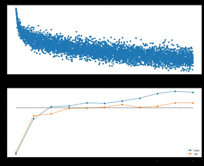
很明显，网络的表现符合50%正确率的要求，并能够从epoch3开始稳定保持

2.3 Multilayer network

实现一个具有任意数量的隐藏层的全连接网络。

class FullyConnectedNet(object):
#2.3.1
    def __init__(
        self,
        hidden_dims,
        input_dim=3 * 32 * 32,
        num_classes=10,
        dropout=1,
        use_batchnorm=False,
        reg=0.0,
        weight_scale=1e-2,
        dtype=np.float32,
        seed=None,
    ):
#use_batchnorm=False
#2.3.2
        self.use_batchnorm = use_batchnorm
        self.use_dropout = dropout != 1
        self.reg = reg
        self.num_layers = 1 + len(hidden_dims)
        self.dtype = dtype
        self.params = {}
#2.3.3
        # *****START OF YOUR CODE (DO NOT DELETE/MODIFY THIS LINE)*****
        # 初始化参数
        for i in range(len(hidden_dims)):
            D = hidden_dims[i]
            self.params['W'+str(i+1)] = weight_scale*np.random.randn(input_dim,D)
            self.params['b'+str(i+1)] = np.zeros(D)
            # 使用BN时，增加两个参数，beta初始化为0（均值），gamma初始化为1（方差）
            if use_batchnorm:
                self.params['gamma'+str(i+1)] = np.ones(D)
                self.params['beta'+str(i+1)] = np.zeros(D)
            input_dim = D
        # 输出层单独写
        self.params['W'+str(self.num_layers)] = weight_scale*np.random.randn(hidden_dims[-1],num_classes)
        self.params['b'+str(self.num_layers)] = np.zeros((num_classes))
#use_batchnorm  
        pass
        # *****END OF YOUR CODE (DO NOT DELETE/MODIFY THIS LINE)*****

#将dropout_param字典传递给每层，以便该层知道dropout的概率和模式
        self.dropout_param = {}
        if self.use_dropout:
            self.dropout_param = {"mode": "train", "p": dropout}
            if seed is not None:
                self.dropout_param["seed"] = seed
#2.3.4
        self.bn_params = []
#        if self.normalization == "batchnorm":
#            self.bn_params = [{"mode": "train"} for i in range(self.num_layers - 1)]
#        if self.normalization == "layernorm":
#            self.bn_params = [{} for i in range(self.num_layers - 1)]
        if self.use_batchnorm:
            self.bn_params = [{'mode': 'train'} for i in xrange(self.num_layers - 1)]
        # Cast all parameters to the correct datatype
        for k, v in self.params.items():
            self.params[k] = v.astype(dtype)

    def loss(self, X, y=None):
 #       Input / output: Same as TwoLayerNet above.
        X = X.astype(self.dtype)
        mode = "test" if y is None else "train"
#为batchnorm参数和dropout参数设置训练/测试模式
#        if self.use_dropout:
#            self.dropout_param["mode"] = mode
        if self.dropout_param is not None:
            self.dropout_param['mode'] = mode         
        if self.use_batchnorm:
#        if self.normalization == "batchnorm":
            for bn_param in self.bn_params:
                bn_param["mode"] = mode
        scores = None
#2.3.5
        # *****START OF YOUR CODE (DO NOT DELETE/MODIFY THIS LINE)*****
#        hidden_layers, caches = list(range(self.num_layers + 1)), list(range(self.num_layers))
        '''创建整数列表（导致“TypeError: ‘range’ object does not support item assignment”）有时你想要得到一个有序的整数列表，所以range() 看上去是生成此列表的不错方式。然而，你需要记住range() 返回的是“range object”，而不是实际的list 值。'''
        cache = {}
        cache_dropout= {}
        input_X = X
        for i in range(self.num_layers-1):            
            W,b = self.params['W'+str(i+1)],self.params['b'+str(i+1)]
            # 如果要用BN，一般是在ReLU层前用
            if self.use_batchnorm:
                gamma,beta = self.params['gamma'+str(i+1)],self.params['beta'+str(i+1)]
                bn_param = self.bn_params[i]
                input_X,cache[i] = affine_bn_relu_forward(input_X,W,b,gamma,beta,bn_param)
            else:
                input_X,cache[i] = affine_relu_forward(input_X,W,b)
            # 如果要用dropout，一般在ReLU后用
            if self.use_dropout:
                input_X,cache_dropout[i] = dropout_forward(input_X,self.dropout_param)
        # 输出层单独写
        W,b = self.params['W'+str(self.num_layers)],self.params['b'+str(self.num_layers)]
        scores,cache[self.num_layers-1] = affine_forward(input_X,W,b)
        pass
        # *****END OF YOUR CODE (DO NOT DELETE/MODIFY THIS LINE)*****

        # If test mode return early
        if mode == "test":
            return scores

        loss, grads = 0.0, {}
     #2.3.6
        # *****START OF YOUR CODE (DO NOT DELETE/MODIFY THIS LINE)*****
        # 输出层单独计算
        loss,dscores = softmax_loss(scores,y)
        W = self.params['W'+str(self.num_layers)]
        loss += self.reg*0.5*np.sum(W**2)        
        dout_relu,dW,db = affine_backward(dscores,cache[self.num_layers-1])
        grads['W'+str(self.num_layers)] = dW+self.reg*W
        grads['b'+str(self.num_layers)] = db        
        
        for i in range(self.num_layers-1,0,-1):
            W = self.params['W'+str(i)]
            loss += self.reg*0.5*np.sum(W**2)
            # dropout层在ReLU层后面，所以先计算它的反向求导
            if self.use_dropout:
                dout_relu = dropout_backward(dout_relu,cache_dropout[i-1])
            # 使用BN时不需要对gamma和beta进行正则化
            if self.use_batchnorm:
                dout_relu,dW,db,dgamma,dbeta = affine_bn_relu_backward(dout_relu,cache[i-1])
                grads['gamma'+str(i)] = dgamma
                grads['beta'+str(i)] = dbeta
            else:
                dout_relu,dW,db = affine_relu_backward(dout_relu,cache[i-1])            
            grads['W'+str(i)] = dW+self.reg*W
            grads['b'+str(i)] = db
   
        pass
        # *****END OF YOUR CODE (DO NOT DELETE/MODIFY THIS LINE)*****
        return loss, grads

代码分析 2.3.1

具有任意数量隐藏层的全连接神经网络
ReLU、softmax损失函数、批处理/图层归一化、Dropout
架构为 {affine - [batch/layer norm] - relu - [dropout]} x (L - 1) - affine - softmax
学习的参数存储在self.params字典，使用Solver类学习。

代码分析 2.3.2

    初始化新的FullyConnectedNet。

    输入：
    -hidden_​​dims：给出每个隐藏层大小的整数列表。
    -input_dim：给出输入大小的整数。
    -num_classes：给出要分类的类数。
    -dropout：介于0和1之间，可提供dropout强度。如果dropout = 1，则网络根本不应该使用dropout。
    -normalization：标准化类型。有效值是“ batchnorm”，“ layernorm”或“无”（不进行标准化）（默认值）。
    -reg：L2正则化强度。
    -weight_scale：权重随机初始化的标准偏差的标量。
    -dtype：一个numpy数据类型对象；所有计算将使用此数据类型执行。使用float64进行数字梯度检查。
    -seed：如果不是“无”，则将此随机种子传递到辍学层。这将使辍学层具有不确定性，因此我们可以对模型进行梯度检查。

代码分析 2.3.3

初始化网络参数，将所有值存储在self.params字典中。 将第一层的权重和偏差存储在W1和b1中； 对于第二层，请使用W2和b2等。权重应从以0为中心的正态分布初始化，标准偏差等于weight_scale。 偏差应初始化为零。
使用批量归一化时，将第一层的缩放和平移参数存储在gamma1和beta1中； 对于第二层，使用gamma2和beta2。Scale参数应初始化为1，shift参数应初始化为零。 

代码分析 2.3.4

使用批处理标准化，需要跟踪均值和方差，因此向每个batchnorm层传递一个特殊的bn_param对象。 
将self.bn_params [0]传递到第一批标准化层的正向传递，将self.bn_params [1]传递给第二批标准化层的正向传递，依此类推。

代码分析 2.3.5

全连接网络实现前向传递，计算X的类分数并将其存储在scores变量中
使用dropout时，将self.dropout_param传递给每个dropout
使用BN时，您需要将self.bn_params [0]传递给第一个BN层的正向传递，将self.bn_params [1]传递给第二个BN层r的正向传递

代码分析 2.3.6

全连接网络实现反向传递。 将损失存储在损失变量中，并将梯度存储在grads词典中。 使用softmax计算loss，并确保grads [k]保持self.params [k]的梯度
使用批处理/图层归一化时，不需要正则化缩放和平移参数。

Test_2.3.1
loss和梯度检查

np.random.seed(231)
N, D, H1, H2, C = 2, 15, 20, 30, 10
X = np.random.randn(N, D)
y = np.random.randint(C, size=(N,))

for reg in [0, 3.14]:
  print('Running check with reg = ', reg)
  model = FullyConnectedNet([H1, H2], input_dim=D, num_classes=C,
                            reg=reg, weight_scale=5e-2, dtype=np.float64)

  loss, grads = model.loss(X, y)
  print('Initial loss: ', loss)
  
  # Most of the errors should be on the order of e-7 or smaller.   
  # NOTE: It is fine however to see an error for W2 on the order of e-5
  # for the check when reg = 0.0
  for name in sorted(grads):
    f = lambda _: model.loss(X, y)[0]
    grad_num = eval_numerical_gradient(f, model.params[name], verbose=False, h=1e-5)
    print('%s relative error: %.2e' % (name, rel_error(grad_num, grads[name])))

输出：

Running check with reg =  0
Initial loss:  2.638793811090764
W1 relative error: 1.57e-08
W2 relative error: 4.68e-08
W3 relative error: 1.45e-06
b1 relative error: 3.94e-10
b2 relative error: 1.23e-10
b3 relative error: 3.68e-10
Running check with reg =  3.14
Initial loss:  451.3464813074225
W1 relative error: 3.12e-07
W2 relative error: 1.39e-06
W3 relative error: 4.72e-08
b1 relative error: 2.08e-08
b2 relative error: 3.45e-08
b3 relative error: 9.95e-08

Test_2.3.2
拟合包含50张图像的小型数据集。 每个隐藏层包含100个单元的三层网络。

# TODO: Use a three-layer Net to overfit 50 training examples by 
# tweaking just the learning rate and initialization scale.

num_train = 50
small_data = {
  'X_train': data['X_train'][:num_train],
  'y_train': data['y_train'][:num_train],
  'X_val': data['X_val'],
  'y_val': data['y_val'],
}

weight_scale = 1e-2   # Experiment with this!
learning_rate = 1e-4  # Experiment with this!
model = FullyConnectedNet([100, 100],
              weight_scale=weight_scale, dtype=np.float64)
solver = Solver(model, small_data,
                print_every=10, num_epochs=20, batch_size=25,
                update_rule='sgd',
                optim_config={
                  'learning_rate': learning_rate,
                }
         )
solver.train()

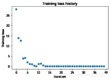
plt.plot(solver.loss_history, 'o')
plt.title('Training loss history')
plt.xlabel('Iteration')
plt.ylabel('Training loss')
plt.show()

输出：

(Iteration 1 / 40) loss: 27.948607
(Epoch 0 / 20) train acc: 0.300000; val_acc: 0.160000
(Epoch 1 / 20) train acc: 0.420000; val_acc: 0.145000
(Epoch 2 / 20) train acc: 0.700000; val_acc: 0.143000
(Epoch 3 / 20) train acc: 0.760000; val_acc: 0.168000
(Epoch 4 / 20) train acc: 0.880000; val_acc: 0.158000
(Epoch 5 / 20) train acc: 0.920000; val_acc: 0.164000
(Iteration 11 / 40) loss: 1.056135
(Epoch 6 / 20) train acc: 0.900000; val_acc: 0.145000
(Epoch 7 / 20) train acc: 0.980000; val_acc: 0.166000
(Epoch 8 / 20) train acc: 0.980000; val_acc: 0.162000
(Epoch 9 / 20) train acc: 1.000000; val_acc: 0.159000
(Epoch 10 / 20) train acc: 1.000000; val_acc: 0.159000
(Iteration 21 / 40) loss: 0.003744
(Epoch 11 / 20) train acc: 1.000000; val_acc: 0.157000
(Epoch 12 / 20) train acc: 1.000000; val_acc: 0.157000
(Epoch 13 / 20) train acc: 1.000000; val_acc: 0.157000
(Epoch 14 / 20) train acc: 1.000000; val_acc: 0.157000
(Epoch 15 / 20) train acc: 1.000000; val_acc: 0.157000
(Iteration 31 / 40) loss: 0.002232
(Epoch 16 / 20) train acc: 1.000000; val_acc: 0.157000
(Epoch 17 / 20) train acc: 1.000000; val_acc: 0.157000
(Epoch 18 / 20) train acc: 1.000000; val_acc: 0.157000
(Epoch 19 / 20) train acc: 1.000000; val_acc: 0.157000
(Epoch 20 / 20) train acc: 1.000000; val_acc: 0.157000

Test_2.3.3
使用每层100个单元的五层网络来拟合50个训练示例。
调整学习率和权重初始化量表

# TODO: Use a five-layer Net to overfit 50 training examples by 
# tweaking just the learning rate and initialization scale.

num_train = 50
small_data = {
  'X_train': data['X_train'][:num_train],
  'y_train': data['y_train'][:num_train],
  'X_val': data['X_val'],
  'y_val': data['y_val'],
}

learning_rate = 1e-3  # Experiment with this!
weight_scale = 3e-2   # Experiment with this!
model = FullyConnectedNet([100, 100, 100, 100],
                weight_scale=weight_scale, dtype=np.float64)
solver = Solver(model, small_data,
                print_every=10, num_epochs=20, batch_size=25,
                update_rule='sgd',
                optim_config={
                  'learning_rate': learning_rate,
                }
         )
solver.train()

plt.plot(solver.loss_history, 'o')
plt.title('Training loss history')
plt.xlabel('Iteration')
plt.ylabel('Training loss')
plt.show()

输出：

(Iteration 1 / 40) loss: 7.981513
(Epoch 0 / 20) train acc: 0.280000; val_acc: 0.133000
(Epoch 1 / 20) train acc: 0.360000; val_acc: 0.111000
(Epoch 2 / 20) train acc: 0.660000; val_acc: 0.158000
(Epoch 3 / 20) train acc: 0.800000; val_acc: 0.148000
(Epoch 4 / 20) train acc: 0.940000; val_acc: 0.146000
(Epoch 5 / 20) train acc: 0.960000; val_acc: 0.138000
(Iteration 11 / 40) loss: 0.189626
(Epoch 6 / 20) train acc: 0.980000; val_acc: 0.138000
(Epoch 7 / 20) train acc: 1.000000; val_acc: 0.141000
(Epoch 8 / 20) train acc: 1.000000; val_acc: 0.140000
(Epoch 9 / 20) train acc: 1.000000; val_acc: 0.148000
(Epoch 10 / 20) train acc: 1.000000; val_acc: 0.149000
(Iteration 21 / 40) loss: 0.088653
(Epoch 11 / 20) train acc: 1.000000; val_acc: 0.146000
(Epoch 12 / 20) train acc: 1.000000; val_acc: 0.150000
(Epoch 13 / 20) train acc: 1.000000; val_acc: 0.150000
(Epoch 14 / 20) train acc: 1.000000; val_acc: 0.153000
(Epoch 15 / 20) train acc: 1.000000; val_acc: 0.152000
(Iteration 31 / 40) loss: 0.033492
(Epoch 16 / 20) train acc: 1.000000; val_acc: 0.150000
(Epoch 17 / 20) train acc: 1.000000; val_acc: 0.151000
(Epoch 18 / 20) train acc: 1.000000; val_acc: 0.152000
(Epoch 19 / 20) train acc: 1.000000; val_acc: 0.153000
(Epoch 20 / 20) train acc: 1.000000; val_acc: 0.153000

三、最优化

实现其他几个更新规则（最优化结构），并且和单纯的SGD做一个比较
原理部分详见：最优化方案

3.1 SGD+Momentum

首先，在optim.py中完善sgd_momentum

def sgd_momentum(w, dw, config=None):
    if config is None:
        config = {}
    config.setdefault("learning_rate", 1e-2)
    config.setdefault("momentum", 0.9)
    v = config.get("velocity", np.zeros_like(w))
    next_w = None
    # *****START OF YOUR CODE (DO NOT DELETE/MODIFY THIS LINE)*****
    v = config['momentum'] * v - config['learning_rate'] * dw
    next_w = w + v
    pass
    # *****END OF YOUR CODE (DO NOT DELETE/MODIFY THIS LINE)*****
    config["velocity"] = v
    return next_w, config

代码分析：

 -learning_rate：学习率。
 -动量：0到1之间给出了动量值
 -速度：与w和dw形状相同的numpy数组，用于存储梯度的移动平均值。
实现动量更新公式。 将更新的值存储在next_w变量

Test_3.1 sgd_momentum

from cs231n.optim import sgd_momentum

N, D = 4, 5
w = np.linspace(-0.4, 0.6, num=N*D).reshape(N, D)
dw = np.linspace(-0.6, 0.4, num=N*D).reshape(N, D)
v = np.linspace(0.6, 0.9, num=N*D).reshape(N, D)

config = {'learning_rate': 1e-3, 'velocity': v}
next_w, _ = sgd_momentum(w, dw, config=config)

expected_next_w = np.asarray([
  [ 0.1406,      0.20738947,  0.27417895,  0.34096842,  0.40775789],
  [ 0.47454737,  0.54133684,  0.60812632,  0.67491579,  0.74170526],
  [ 0.80849474,  0.87528421,  0.94207368,  1.00886316,  1.07565263],
  [ 1.14244211,  1.20923158,  1.27602105,  1.34281053,  1.4096    ]])
expected_velocity = np.asarray([
  [ 0.5406,      0.55475789,  0.56891579, 0.58307368,  0.59723158],
  [ 0.61138947,  0.62554737,  0.63970526,  0.65386316,  0.66802105],
  [ 0.68217895,  0.69633684,  0.71049474,  0.72465263,  0.73881053],
  [ 0.75296842,  0.76712632,  0.78128421,  0.79544211,  0.8096    ]])

# Should see relative errors around e-8 or less
print('next_w error: ', rel_error(next_w, expected_next_w))
print('velocity error: ', rel_error(expected_velocity, config['velocity']))

输出：

next_w error:  8.882347033505819e-09
velocity error:  4.269287743278663e-09

SGD与SGD+Momentum的对比略，直观看出SGD+Momentum的优势，收敛更快，效果更好

3.2 RMSProp

def rmsprop(w, dw, config=None):
    if config is None:
        config = {}
    config.setdefault("learning_rate", 1e-2)
    config.setdefault("decay_rate", 0.99)
    config.setdefault("epsilon", 1e-8)
    config.setdefault("cache", np.zeros_like(w))
    next_w = None
    # *****START OF YOUR CODE (DO NOT DELETE/MODIFY THIS LINE)*****
    config['cache'] = config['decay_rate'] * config['cache'] + (1 - config['decay_rate']) * dw ** 2
    next_w = w - config['learning_rate'] * dw / (np.sqrt(config['cache']) + config['epsilon'])    
    pass
    # *****END OF YOUR CODE (DO NOT DELETE/MODIFY THIS LINE)*****
    return next_w, config

代码分析：

 RMSProp，使用平方移动平均值

 配置格式：
 -learning_rate：学习率。
 -delay_rate：0到1之间，给出平方的衰减率
 -epsilon：小标量，用于平滑以避免除以零。
 -cache

Test_3.2 rmsprop

# Test RMSProp implementation
from cs231n.optim import rmsprop

N, D = 4, 5
w = np.linspace(-0.4, 0.6, num=N*D).reshape(N, D)
dw = np.linspace(-0.6, 0.4, num=N*D).reshape(N, D)
cache = np.linspace(0.6, 0.9, num=N*D).reshape(N, D)

config = {'learning_rate': 1e-2, 'cache': cache}
next_w, _ = rmsprop(w, dw, config=config)

expected_next_w = np.asarray([
  [-0.39223849, -0.34037513, -0.28849239, -0.23659121, -0.18467247],
  [-0.132737,   -0.08078555, -0.02881884,  0.02316247,  0.07515774],
  [ 0.12716641,  0.17918792,  0.23122175,  0.28326742,  0.33532447],
  [ 0.38739248,  0.43947102,  0.49155973,  0.54365823,  0.59576619]])
expected_cache = np.asarray([
  [ 0.5976,      0.6126277,   0.6277108,   0.64284931,  0.65804321],
  [ 0.67329252,  0.68859723,  0.70395734,  0.71937285,  0.73484377],
  [ 0.75037008,  0.7659518,   0.78158892,  0.79728144,  0.81302936],
  [ 0.82883269,  0.84469141,  0.86060554,  0.87657507,  0.8926    ]])

# You should see relative errors around e-7 or less
print('next_w error: ', rel_error(expected_next_w, next_w))
print('cache error: ', rel_error(expected_cache, config['cache']))

输出：

next_w error:  9.524687511038133e-08
cache error:  2.6477955807156126e-09

3.3 Adam

def adam(w, dw, config=None):
    if config is None:
        config = {}
    config.setdefault("learning_rate", 1e-3)
    config.setdefault("beta1", 0.9)
    config.setdefault("beta2", 0.999)
    config.setdefault("epsilon", 1e-8)
    config.setdefault("m", np.zeros_like(w))
    config.setdefault("v", np.zeros_like(w))
    config.setdefault("t", 1)

    next_w = None  
    # *****START OF YOUR CODE (DO NOT DELETE/MODIFY THIS LINE)*****
    bt1 = config['beta1']
    bt2 = config['beta2']
    t = config['t']
    lr = config['learning_rate']    
    
    config['m'] = bt1*config['m'] + (1-bt1)*dw
    mt = config['m']/(1-bt1**t)
    config['v'] = bt2*config['v'] + (1-bt2)*dw**2
    vt = config['v']/(1-bt2**t)
    next_w = w - lr*mt/(np.sqrt(vt)+config['epsilon'])
    config['t'] += 1 
    pass
    # *****END OF YOUR CODE (DO NOT DELETE/MODIFY THIS LINE)*****
    return next_w, config

代码分析：

 Adam规则合并了渐变及其平方的移动平均值以及偏差校正项。

 配置格式：
 -learning_rate：学习率。
 -beta1：梯度第一矩移动平均值的衰减率。
 -beta2：梯度第二矩的移动平均值的衰减率。
 -epsilon：小标量，用于平滑以避免除以零。
 -m：梯度的移动平均值
 -v：平方梯度的移动平均值
 -t：迭代次数

注意，在这里一定处理好 t=0的情况，实时更新m、v、t

Test_3.3 Adam

# Test Adam implementation
from cs231n.optim import adam

N, D = 4, 5
w = np.linspace(-0.4, 0.6, num=N*D).reshape(N, D)
dw = np.linspace(-0.6, 0.4, num=N*D).reshape(N, D)
m = np.linspace(0.6, 0.9, num=N*D).reshape(N, D)
v = np.linspace(0.7, 0.5, num=N*D).reshape(N, D)

config = {'learning_rate': 1e-2, 'm': m, 'v': v, 't': 5}
next_w, _ = adam(w, dw, config=config)

expected_next_w = np.asarray([
  [-0.40094747, -0.34836187, -0.29577703, -0.24319299, -0.19060977],
  [-0.1380274,  -0.08544591, -0.03286534,  0.01971428,  0.0722929],
  [ 0.1248705,   0.17744702,  0.23002243,  0.28259667,  0.33516969],
  [ 0.38774145,  0.44031188,  0.49288093,  0.54544852,  0.59801459]])
expected_v = np.asarray([
  [ 0.69966,     0.68908382,  0.67851319,  0.66794809,  0.65738853,],
  [ 0.64683452,  0.63628604,  0.6257431,   0.61520571,  0.60467385,],
  [ 0.59414753,  0.58362676,  0.57311152,  0.56260183,  0.55209767,],
  [ 0.54159906,  0.53110598,  0.52061845,  0.51013645,  0.49966,   ]])
expected_m = np.asarray([
  [ 0.48,        0.49947368,  0.51894737,  0.53842105,  0.55789474],
  [ 0.57736842,  0.59684211,  0.61631579,  0.63578947,  0.65526316],
  [ 0.67473684,  0.69421053,  0.71368421,  0.73315789,  0.75263158],
  [ 0.77210526,  0.79157895,  0.81105263,  0.83052632,  0.85      ]])

# You should see relative errors around e-7 or less
print('next_w error: ', rel_error(expected_next_w, next_w))
print('v error: ', rel_error(expected_v, config['v']))
print('m error: ', rel_error(expected_m, config['m']))

输出：

next_w error:  0.0015218451757856217
v error:  4.208314038113071e-09
m error:  4.214963193114416e-09

3.4 四种优化方式的比较

learning_rates = {'rmsprop': 1e-4, 'adam': 1e-3}
for update_rule in ['adam', 'rmsprop']:
  print('running with ', update_rule)
  model = FullyConnectedNet([100, 100, 100, 100, 100], weight_scale=5e-2)

  solver = Solver(model, small_data,
                  num_epochs=5, batch_size=100,
                  update_rule=update_rule,
                  optim_config={
                    'learning_rate': learning_rates[update_rule]
                  },
                  verbose=True)
  solvers[update_rule] = solver
  solver.train()
  print()

plt.subplot(3, 1, 1)
plt.title('Training loss')
plt.xlabel('Iteration')

plt.subplot(3, 1, 2)
plt.title('Training accuracy')
plt.xlabel('Epoch')

plt.subplot(3, 1, 3)
plt.title('Validation accuracy')
plt.xlabel('Epoch')

for update_rule, solver in list(solvers.items()):
  plt.subplot(3, 1, 1)
  plt.plot(solver.loss_history, 'o', label=update_rule)
  
  plt.subplot(3, 1, 2)
  plt.plot(solver.train_acc_history, '-o', label=update_rule)

  plt.subplot(3, 1, 3)
  plt.plot(solver.val_acc_history, '-o', label=update_rule)
  
for i in [1, 2, 3]:
  plt.subplot(3, 1, i)
  plt.legend(loc='upper center', ncol=4)
plt.gcf().set_size_inches(15, 15)
plt.show()

输出：

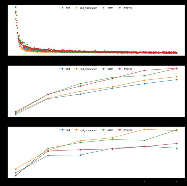
具体数值略，但很明显adam表现不错（千万千万看好 t ）

四、训练和预测

4.1 Train

训练一个全连接模型（我这里设计了一个简单的5层模型，没有使用BN和Dropout）
调试出最优参数后，就把循环注释掉了

best_model = None
# *****START OF YOUR CODE (DO NOT DELETE/MODIFY THIS LINE)*****
best_val = -1
best_solver = None

from copy import deepcopy
learning_rates = 3.1e-4
weight_scales = [2.5e-2]
for ws in weight_scales:
#    for lr in learning_rates:
        model = FullyConnectedNet([500, 400, 300, 200, 100], weight_scale=ws)
        print('weight_scales:%e learning_rate:%e'%(ws,lr))
        
        solver = Solver(model, data,
                  print_every=500,num_epochs=10, batch_size=100,
                  update_rule='adam',
                  optim_config={
                    'learning_rate': lr
                  },
                  verbose=True)
        
        solver.train()
        if solver.best_val_acc>best_val:
            best_val = solver.best_val_acc
            best_solver = deepcopy(solver)
            best_model = model
            print(lr,ws)
        print()
# 得到的最好超参数weight_scales:2.5e-02 learning_rate:3.1e-04
pass
# *****END OF YOUR CODE (DO NOT DELETE/MODIFY THIS LINE)*****

输出：

weight_scales:2.500000e-02 learning_rate:3.100000e-04
(Iteration 1 / 4900) loss: 9.108568
(Epoch 0 / 10) train acc: 0.108000; val_acc: 0.114000
(Epoch 1 / 10) train acc: 0.460000; val_acc: 0.440000
(Iteration 501 / 4900) loss: 1.504805
(Epoch 2 / 10) train acc: 0.511000; val_acc: 0.457000
(Iteration 1001 / 4900) loss: 1.436040
(Epoch 3 / 10) train acc: 0.550000; val_acc: 0.469000
(Iteration 1501 / 4900) loss: 1.325850
(Epoch 4 / 10) train acc: 0.557000; val_acc: 0.488000
(Iteration 2001 / 4900) loss: 1.141446
(Epoch 5 / 10) train acc: 0.574000; val_acc: 0.489000
(Iteration 2501 / 4900) loss: 1.084415
(Epoch 6 / 10) train acc: 0.595000; val_acc: 0.505000
(Iteration 3001 / 4900) loss: 1.319046
(Epoch 7 / 10) train acc: 0.637000; val_acc: 0.516000
(Iteration 3501 / 4900) loss: 1.013175
(Epoch 8 / 10) train acc: 0.697000; val_acc: 0.516000
(Iteration 4001 / 4900) loss: 1.133661
(Epoch 9 / 10) train acc: 0.654000; val_acc: 0.537000
(Iteration 4501 / 4900) loss: 1.045279
(Epoch 10 / 10) train acc: 0.719000; val_acc: 0.522000
0.00031 0.025

4.2 Test_final

y_test_pred = np.argmax(best_model.loss(data['X_test']), axis=1)
y_val_pred = np.argmax(best_model.loss(data['X_val']), axis=1)
print('Validation set accuracy: ', (y_val_pred == data['y_val']).mean())
print('Test set accuracy: ', (y_test_pred == data['y_test']).mean())

输出：

Validation set accuracy:  0.537
Test set accuracy:  0.518

虽然没有达到55%，但是已经是个不错的成绩

五、问题

Inline Question 1:

提问：We’ve only asked you to implement ReLU, but there are a number of different activation functions that one could use in neural networks, each with its pros and cons. In particular, an issue commonly seen with activation functions is getting zero (or close to zero) gradient flow during backpropagation. Which of the following activation functions have this problem? If you consider these functions in the one dimensional case, what types of input would lead to this behaviour?
Sigmoid、ReLU、Leaky ReLU

翻译：我们仅要求您实现ReLU，但是神经网络可以使用许多不同的激活函数，每种都有其优缺点。 特别地，激活函数通常会遇到的一个问题是在反向传播期间获得零（或接近零）的梯度流。 以下哪个激活功能有此问题？ 如果在一维的情况下考虑这些功能，哪种输入会导致这种行为？

回答：

Inline Question 2:

提问：Did you notice anything about the comparative difficulty of training the three-layer net vs training the five layer net? In particular, based on your experience, which network seemed more sensitive to the initialization scale? Why do you think that is the case?

翻译：您是否注意到训练三层网络与训练五层网络的相对难度？ 特别是，根据您的经验，哪个网络似乎对初始化规模更敏感？ 您为什么认为是这种情况？

回答：

Inline Question 3:

AdaGrad, like Adam, is a per-parameter optimization method that uses the following update rule:

cache += dw**2
w += - learning_rate * dw / (np.sqrt(cache) + eps)

John notices that when he was training a network with AdaGrad that the updates became very small, and that his network was learning slowly. Using your knowledge of the AdaGrad update rule, why do you think the updates would become very small? Would Adam have the same issue?