论文笔记 A theory of learning from different domains

domain adaptation 领域理论方向的重要论文. 这篇笔记主要是推导文章中的定理, 还有分析定理的直观解释. 笔记中的章节号与论文中的保持一致.

1. Introduction

domain adaptation 的设定介绍:
有两个域, source domain 与 target domain.
source domain: 一组从 source dist. 采样的带有标签的数据.
target domain: 一组从 target dist. 采样的无标签的数据, 或者有很少的数据带标签.
其中 source dist. $\ne$ target dist.
目标: 学习一个能在 target domian 上表现得好的模型.
(第二节跳过)

3. A rigorous model of domain adaptation

首先关注二分类问题. 这节主要是给出了本文中用到的一些notations.

• $<{\mathcal{D}}_S,f_S>$ 表示 source domain, 前者是 source dist, 后者是 source dist. 上的 ground truth function.
• $<{\mathcal{D}}_T,f_T>$ 表示 target domain, 同上.
• $h:\mathcal{X}\to \{0,1\}$ 表示一个从输入空间映射到二分类集合的 hypothesis.
• 在分布 ${\mathcal{D}}_S$ 上, 两个 hypotheses $h$ 与 $f$ 的平均差异定义为:
  $${ϵ}_S(h,f)={\mathbf{E}}_{x\sim {\mathcal{D}}_S}[|h(x)-f(x)|]$$
  由于 $h$ 与 $f$ 的输出是 0 或 1, 所以只有它们输出不同时, 期望中间的部分为 1, 所以上式为两个hypotheses之间的平均差异(或 disagreements).
• source error of $h$: ${ϵ}_S(h)={ϵ}_S(h,f_S)$, 也就是 $h$ 在source domain 上的错误率 (generalization error).
• empirical source error of $h$: ${\widehat{ϵ}}_S(h)$, 也就是 $h$ 在source domain 上的经验错误率 (empirical error).
• 相同的, 在 target domain 上的 notations: ${ϵ}_T(h,f),{ϵ}_T(h),$ 和${\widehat{ϵ}}_T(h)$.

4. A bound relating the source and target error

现在, 想要分析一个在 source domian 上训练的分类器在 target domian 上的 generalization error (即 ${ϵ}_T(h)$) 是多少. 这个值肯定无法计算出来, 所以最直观的想法就是用 source error (即 ${ϵ}_S(h)$) 和 两个域之间的差异来 bound target error.
那么用什么来表示两个域之间的差异呢? 文章首先用 $L^1$ Divergence 表示这个差异, 并给出了用$L^1$ Divergence 的 bound.
但是 $L^1$ Divergence 有很多缺点, 所以作者提出了第二种方法来表示域之间的差异 – $\mathcal{H}$ Divergence, 为了给出相应的 bound, 又将 $\mathcal{H}$ Divergence 扩展成 $\mathcal{H}\Delta \mathcal{H}$ Divergence.

a) $L^1$ Divergence

也叫 Variation Divergence, Variation Distance, TV Distance.
$$d_1(\mathcal{D},{\mathcal{D}}^{\prime })=2\underset{B\in \mathcal{B}}{\sup }|\underset{\mathcal{D}}{\mathrm{Pr}}[B]-\underset{{\mathcal{D}}^{\prime }}{\mathrm{Pr}}[B]|$$
其中 $\mathcal{B}$ 是在 $\mathcal{D}$ 和 ${\mathcal{D}}^{\prime }$ 上所有可测子集的集合.
用两个很简单的一维分布来表示一下:

上面两个: $\mathcal{B}=[x_1,x_3]\vee [x_2,x_4]=[x_1,x_4]$. 红色区域和蓝色区域的面积是相等的, 因为面积就是概率. 很明显, 对于这两种情况而言, $d_1(\mathcal{D},{\mathcal{D}}^{\prime })$ 就等于2倍蓝色区域面积=2倍红色面积=蓝色面积+红色面积.
下面两个: 两个分布没有重合区域, $d_1(\mathcal{D},{\mathcal{D}}^{\prime })$ 等于2倍的 $\mathcal{D}$ 的面积=2倍的 ${\mathcal{D}}^{\prime }$ 的面积=2. 这里很容易发现, 无论 $\mathcal{D}$ 与 ${\mathcal{D}}^{\prime }$ 相隔多远, 差异多大, 只要它们没有重合部分, $d_1(\mathcal{D},{\mathcal{D}}^{\prime })$ 永远等于2.
从上图还能得出一个公式:
$$d_1(\mathcal{D},{\mathcal{D}}^{\prime })=||\mathcal{D}-{\mathcal{D}}^{\prime }|{|}_1=\int |\mathcal{D}(x)-{\mathcal{D}}^{\prime }(x)|dx$$
其中 $\mathcal{D}(x)$ 表示 $\mathcal{D}$ 的 pdf.

Thm1. 对于任意一个 hypothesis $h$,
$${ϵ}_T(h)\le {ϵ}_S(h)+d_1({\mathcal{D}}_S,{\mathcal{D}}_T)+\min \{{\mathbf{E}}_{{\mathcal{D}}_S}[|f_S(x)-f_T(x)|],{\mathbf{E}}_{{\mathcal{D}}_T}[|f_S(x)-f_T(x)|]\}$$
证明:

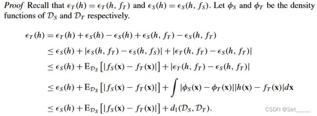
上图是文章给的证明, 前四行很好理解, 解释下最后一行:
$$\int |{\varphi }_S(x)-{\varphi }_T(x)||h(x)-f_T(x)|dx\le \int |{\varphi }_S(x)-{\varphi }_T(x)|dx=d_1(\mathcal{D},{\mathcal{D}}^{\prime })$$
其中 $|h(x)-f_T(x)|\le 1$, $\int |{\varphi }_S(x)-{\varphi }_T(x)|dx=d_1(\mathcal{D},{\mathcal{D}}^{\prime })$ 在前面讲过. 这里再一次体现了前面提到的缺点, 只要不同, 无论$h,f_T$ 有多远 $|h(x)-f_T(x)|$都等于1.
用 $L^1$ Divergence 来做 bound 有以下两个缺点: 1) 无法从有限的样本来估计; 2) bound 很松.

b) $\mathcal{H}$ Divergence

Def. 1 给定在输入空间 $\mathcal{X}$ 上的两个概率分布 $\mathcal{D}$ 和 ${\mathcal{D}}^{\prime }$, $\mathcal{H}$ 表示 $\mathcal{X}$上的hypothesis space, $I(h)$ 为指示函数(即$x\in I(h)\iff h(x)=1$). 那么, $\mathcal{D}$ 和 ${\mathcal{D}}^{\prime }$ 之间的 $\mathcal{H}$ divergence 为:
$$d_{\mathcal{H}}(\mathcal{D},{\mathcal{D}}^{\prime })=2\underset{h\in \mathcal{H}}{\sup }|{\text{Pr}}_{\mathcal{D}}[I(h)]-{\text{Pr}}_{{\mathcal{D}}^{\prime }}[I(h)]|$$
$I(h)$ 可以理解为 $h$ 将输入空间分类成 $1$ 的那部分集合, i.e. $I(h)=\{x|h(x)=1\}$. 所以 $d_{\mathcal{H}}$ 就是 $I(h)$ 在分布 $\mathcal{D}$ 和 ${\mathcal{D}}^{\prime }$ 上的概率之差, 其中注意 $\sup$ over all $h\in \mathcal{H}$, 也就是选取令概率之差最大的那个假设 $h$.
$\mathcal{H}$ Divergence 的好处是: 1) 可以使用有限的样本来估计, 也就是 $d_{\mathcal{H}}$ 可以用 ${\hat{d}}_{\mathcal{H}}$ 来近似. 文章给出了 Lemma 2 和 Lemma 1, 分别为 ${\hat{d}}_{\mathcal{H}}$ 的计算公式和使用 VC dimension 作为复杂度计算 $d_{\mathcal{H}}$ 与 ${\hat{d}}_{\mathcal{H}}$ 的 bound . 2) $d_{\mathcal{H}}\le d_1$.
这里 empirical 版本的计算与估计并不重要, 使用不同的复杂度可以得到不同的 bound 方式, 所以跳过 Lemma 1,2.

c) $\mathcal{H}\Delta \mathcal{H}$ Divergence

首先给出一个定义:
Def. 2: $h^{\ast }$ 为 ideal joint hypothesis, 它最小化了源域和目标域的联合误差(combined error). 用 $\lambda$ 表示相对应的combined error:

$$\begin{gathered} h^{\ast }=\arg \underset{h\in \mathcal{H}}{\min }\{{ϵ}_S(h)+{ϵ}_T(h)\} \\ \lambda ={ϵ}_S(h^{\ast })+{ϵ}_T(h^{\ast }) \end{gathered}$$
然后给出一个新的 hypothesis space: $\mathcal{H}\Delta \mathcal{H}$
Def.3 对于一个 hypothesis space $\mathcal{H}$, 它相对应的 $\mathcal{H}\Delta \mathcal{H}$ 空间为:
$$g\in \mathcal{H}\Delta \mathcal{H}\iff g(x)=h(x)\oplus h^{\prime }(x)\text{ for some }h,h^{\prime }\in \mathcal{H}$$
举个一维输入空间的简单例子: 考虑这样的一个 hypothesis class:
$$\begin{gathered} \mathcal{H}:=\{h_{\alpha }:\alpha \in \mathbb{R}\}. \\ {h}_{\alpha }(x)=\{\begin{array}{cc}1,& \alpha \ge \alpha \\ 0,& \alpha <\alpha \end{array} \end{gathered}$$
那么, 它相应的 $\mathcal{H}\Delta \mathcal{H}$ 空间就是:
$$\begin{gathered} \mathcal{H}\Delta \mathcal{H}=\{g_{{\alpha }_1,{\alpha }_2}:{\alpha }_1,{\alpha }_2\in \mathbb{R}\}. \\ {g}_{{\alpha }_1,{\alpha }_2}=\{\begin{array}{cc}1,& x\in ({\alpha }_1,{\alpha }_2)\\ 0,& o.w.\end{array} \end{gathered}$$
这时, 将 $\mathcal{H}$ Divergence 中的假设空间换成 $\mathcal{H}\Delta \mathcal{H}$ 空间, 就得出了 $\mathcal{H}\Delta \mathcal{H}$ Divergence. 如果按照定义从头推算一遍就是:
$$\begin{gathered} d_{\mathcal{H}\Delta \mathcal{H}}({\mathcal{D}}_S,{\mathcal{D}}_T)=2\underset{g\in \mathcal{H}\Delta \mathcal{H}}{\sup }|\underset{{\mathcal{D}}_S}{\mathrm{Pr}}[I(g)]-\underset{{\mathcal{D}}_T}{\mathrm{Pr}}[I(g)]| \\ =2\underset{h,h^{\prime }\in \mathcal{H}}{\sup }|\underset{x\sim {\mathcal{D}}_S}{\mathrm{Pr}}[h(x)\ne h^{\prime }(x)]-\underset{x\sim {\mathcal{D}}_T}{\mathrm{Pr}}[h(x)\ne h^{\prime }(x)]| \\ =2\underset{h,h^{\prime }\in \mathcal{H}}{\sup }|{ϵ}_S(h,h^{\prime })-{ϵ}_T(h,h^{\prime })| \end{gathered}$$
其中第二行是因为, $I(g)$ 即为 $g(x)=1$ 的那部分输入空间的集合, 由 Def.3 可知, $g(x)=1$ 等价于 $h(x)\ne h^{\prime }(x)$, 虽然不知道具体哪个 $h,h^{\prime }$, 但只关心在假设空间中令概率差值最大的那两个.

这同时也十分直观的得到了 Lemma 3:
对任意两个 hypotheses $h,h^{\prime }$,
$$|{ϵ}_S(h,h^{\prime })-{ϵ}_T(h,h^{\prime })|\le \frac{1}{2}{d}_{\mathcal{H}\Delta \mathcal{H}}(D_S,D_T)$$
有了以上信息, 我们可以用$d_{\mathcal{H}\Delta \mathcal{H}}$给出 ${ϵ}_T$ 的上界:
Thm.2: $\mathcal{H}$ 为 VC-dim = d 的假设空间, ${\mathcal{U}}_S,{\mathcal{U}}_T$ 为来自于 ${\mathcal{D}}_S,{\mathcal{D}}_T$ 的, 大小为 $m^{\prime }$ 的样本. 那么对于任意的 $\delta \in (0,1)$ 和任意的 $h\in \mathcal{H}$ , 以下不等式至少 $1-\delta$ 的概率成立:

$$\begin{gathered} {ϵ}_T(h)\le {ϵ}_S(h)+\frac{1}{2}{d}_{\mathcal{H}\Delta \mathcal{H}}({\mathcal{D}}_S,{\mathcal{D}}_T)+\lambda \\ \le {ϵ}_S(h)+\frac{1}{2}{\hat{d}}_{\mathcal{H}\Delta \mathcal{H}}(U_S,U_T)+4\sqrt{\frac{2d\log (2m^{\prime })+\log (\frac{2}{\delta })}{m^{\prime }}}+\lambda \end{gathered}$$
同样的, 先忽略 empircal 的那部分, 也就是看不等式的第一行. $d_{\mathcal{H}\Delta \mathcal{H}}({\mathcal{D}}_S,{\mathcal{D}}_T)$ 表示了两个域的分布之间的差异, 同时与 $\mathcal{H}$ 有关. $\lambda$ 表示的是 $\mathcal{H}$ 在两个域上最小的联合错误率, 其实也蕴含了两个域分布之间的关系, 同时又与 $\mathcal{H}$ 有关. 所以 ${ϵ}_T(h)-{ϵ}_S(h)$ 用 $d_{\mathcal{H}\Delta \mathcal{H}}({\mathcal{D}}_S,{\mathcal{D}}_T)$ 和 $\lambda$ 进行 bound 很合理.
证明十分简单, 主要就是用到 triangle inequality, 文章中也给出了完整的证明过程, 这里就不粘贴了.

5. A learning bound combining source and target training data

现在考虑这样的学习模式:
训练集为 $S=(S_T,S_S)$, 其中 $S_T$ 为 $\beta m$ 个从分布 ${\mathcal{D}}_T$ 中独立抽取的实例, $S_S$ 为 $(1-\beta )m$ 个从分布 ${\mathcal{D}}_S$ 中独立抽取的实例. 学习的目标是寻找一个 $h$ 以最小化 ${ϵ}_T(h)$. 这里考虑使用 ERM, 但 Domain adaptation 任务中 $\beta$ 往往很小, 所以直接最小化 target error 不合适. 作者考虑在训练过程中, 最小化 source error 和 target error 的和:
$${\widehat{ϵ}}_{\alpha }(h)=\alpha {\widehat{ϵ}}_T(h)+(1-\alpha ){\widehat{ϵ}}_S(h)$$
其中 $\alpha \in [0,1]$. 接下来, 文章给出了两个 定理, 分别为 ${ϵ}_T(h)$ 与 ${ϵ}_{\alpha }(h)$ 之间的bound (Lemma 4) 和 ${ϵ}_{\alpha }(h)$ 与 ${\widehat{ϵ}}_{\alpha }(h)$ 之间的 bound (Lemma 5).

Lemma. 4:
对于任意一个 $h\in \mathcal{H}$,
$$|{ϵ}_{\alpha }(h)-{ϵ}_T(h)|\le (1-\alpha )\left(\frac{1}{2}{d}_{\mathcal{H}\Delta \mathcal{H}}(D_S,D_T)+\lambda \right)$$
证明同样依赖于 用到 triangle inequality:

而且如果把 Lemma 4 左边的 ${ϵ}_{\alpha }$ 展开, 再左右两边消掉 $(1-\alpha )$, 此时 Lemma 4 与 Thm.2 其实是等价的.

Lemma 5: 对于一个 hypothesis $h$, 如果训练样本是由 $\beta m$ 个从分布 ${\mathcal{D}}_T$ 中独立抽取的实例和 $(1-\beta )m$ 个从分布 ${\mathcal{D}}_S$ 中独立抽取的实例构成的, 且这些实例被 $f_S,f_T$ 打上标签. 那么, 对于任何的 $\delta \in (0,1)$, 下式至少有 $1-\delta$ 的概率成立:
$$\mathrm{Pr}[|{\widehat{ϵ}}_{\alpha }(h)-{ϵ}_{\alpha }(h)|\ge ϵ]\le \exp [\frac{-2m{ϵ}^2}{\frac{{\alpha }^2}{\beta }+\frac{(1-\alpha {)}^2}{1-\beta }}]$$
证明依赖于 Hoeffding Inequality, 我在这篇博客中给了 2) Chernoff bound, Hoeffding’s Lemma, Hoeffding’s inequality 定理的介绍和推导.
证明:
按 ${\widehat{ϵ}}_{\alpha }$ 的定义和 empirical error 的定义展开, 有:

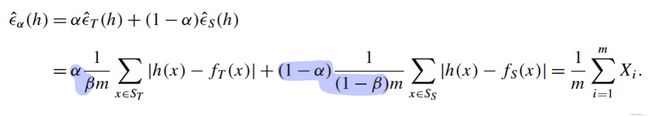
这个形式就很容易观察了.
令 $X_1,...,X_{\beta m}$ 表示值为 $\frac{\alpha }{\beta }|h(x)-f_T(x)|$ 的随机变量.
令 $X_{\beta m+1},...,X_m$ 表示值为 $\frac{1-\alpha }{1-\beta }|h(x)-f_S(x)|$ 的随机变量.
那么, 很容易计算出 ${\widehat{ϵ}}_{\alpha }(h)=\frac{1}{m}{\sum }_{i=1}^m{X}_i$ , 且 $\mathbf{E}[{\widehat{ϵ}}_{\alpha }(h)]={ϵ}_{\alpha }(h)$, 所以直接应用 Hoeffding Inequality 就得到 Lemma 5 的不等式.

未完待续.