R语言 假设检验(非参数) 学习笔记
1.皮尔森拟合优度塔防检验。
假设H0:总体具有某分布F 备择假设H1:总体不具有该分布。
我们将数轴分成若干个区间,所抽取的样本会分布在这些区间中。在原假设成立的条件下,我们便知道每个区间包含样本的个数的期望值。用实际值Ni 与期望值Npi可以构造统计量K 。皮尔森证明,n趋向于无穷时,k收敛于m-1的塔防分布。m为我们分组的个数。有了这个分布,我们就可以做假设检验。
例:
#如果是均匀分布,则没有明显差异 。这里组其实已经分好了,直接用 。H0:人数服从均匀分布
> x <- c(210,312,170,85,223)
> n <- sum(x); m <- length(x)
> p <- rep(1/m,m)
> K <- sum((x-n*p)^2/(n*p)); K #计算出K值
[1] 136.49
> p <- 1-pchisq(K,m-1); p #计算出p值
[1] 0 #拒绝原假设。
在R语言中 chisq.test(),可以完成拟合优度检验。默认就是检验是否为均匀分布,如果是其他分布,需要自己分组,并在参数p中指出。上面题目的解法
chisq.test(x)

        Chi-squared test for given probabilities

data:  x
X-squared = 136.49, df = 4, p-value < 2.2e-16 #同样拒绝原假设。
例,用这个函数检验其他分布。 抽取31名学生的成绩,检验是否为正态分布。
> x <- c(25,45,50,54,55,61,64,68,72,75,75,78,79,81,83,84,84,84,85,
86,86,86,87,89,89,89,90,91,91,92,100)
> A <- table(cut(x,breaks=c(0,69,79,89,100))) #对样本数据进行分组。
> A

  (0,69]  (69,79]  (79,89] (89,100]
       8        5       13        5
> p <- pnorm(c(70,80,90,100),mean(x),sd(x)) #获得理论分布的概率值
> p <- c(p[1],p[2]-p[1],p[3]-p[2],1-p[3])
> chisq.test(A,p=p)

        Chi-squared test for given probabilities

data:  A
X-squared = 8.334, df = 3, p-value = 0.03959  #检验结果不是正态的。
例:大麦杂交后关于芒性的比例应该是 无芒:长芒:短芒=9:3:4 。 我们的实际观测值是335:125:160 。请问观测值是否符合预期?
> p <- c(9/16,3/16,4/16)
> x <- c(335,125,160)
> chisq.test(x,p=p)

        Chi-squared test for given probabilities

data:  x
X-squared = 1.362, df = 2, p-value = 0.5061
在分组的时候要注意,每组的频数要大于等于5.
如果理论分布依赖于多个未知参数,只能先由样本得到参数的估计量。然后构造统计量K,此时K的自由度减少位置参数的数量个。
2.ks检验。
R语言中提供了ks.test()函数,理论上可以检验任何分布。他既能够做单样本检验,也能做双样本检验。
单样本 例:记录一台设备无故障工作时常,并从小到大排序420 500 920 1380 1510 1650 1760 2100 2300 2350。问这些时间是否服从拉姆达=1/1500的指数分布?
> x <- c(420,500,920,1380,1510,1650,1760,2100,2300,2350)
> ks.test(x,"pexp",1/1500)

        One-sample Kolmogorov-Smirnov test

data:  x
D = 0.3015, p-value = 0.2654
alternative hypothesis: two-sided
双样本 例:有两个分布,分别抽样了一些数据,问他们是否服从相同的分布。
> X<-scan()
1: 0.61 0.29 0.06 0.59 -1.73 -0.74 0.51 -0.56 0.39
10: 1.64 0.05 -0.06 0.64 -0.82 0.37 1.77 1.09 -1.28
19: 2.36 1.31 1.05 -0.32 -0.40 1.06 -2.47
26:
Read 25 items
> Y<-scan()
1: 2.20 1.66 1.38 0.20 0.36 0.00 0.96 1.56 0.44
10: 1.50 -0.30 0.66 2.31 3.29 -0.27 -0.37 0.38 0.70
19: 0.52 -0.71
21:
Read 20 items
> ks.test(X,Y)

        Two-sample Kolmogorov-Smirnov test #原假设为 他们的分布相同

data:  X and Y
D = 0.23, p-value = 0.5286
alternative hypothesis: two-sided
3.列联表数据独立性检验。
chisq.test() 同样可以做列联表数据独立性检验,只要将数据写成矩阵的形式就可以了。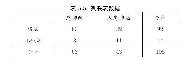
> x <- matrix(c(60,3,32,11),nrow=2) #参数correct是逻辑变量 表示带不带连续矫正。
> x
     [,1] [,2]
[1,]   60   32
[2,]    3   11
> chisq.test(x)

        Pearson's Chi-squared test with Yates' continuity correction

data:  x
X-squared = 7.9327, df = 1, p-value = 0.004855  #拒绝假设 认为有关系
如果一个单元格内的数据小于5 那么做pearson检验是无效的。此时应该使用Fisher精确检验。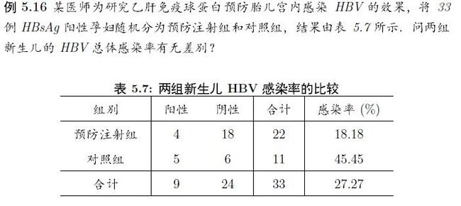
> x <- matrix(c(4,5,18,6),nrow=2)
> x
     [,1] [,2]
[1,]    4   18
[2,]    5    6
> fisher.test(x)

        Fisher's Exact Test for Count Data

data:  x
p-value = 0.121
alternative hypothesis: true odds ratio is not equal to 1
95 percent confidence interval:
 0.03974151 1.76726409  #p值大与0.05, 区间估计包含1,所以认为没有关系。
sample estimates:
odds ratio
 0.2791061
McNemar检验。这个不是相关性检验。是配对卡放检验。也就是说,我们是对一个样本做了两次观测,本身不是独立的样本而是相关的样本,而我们检验的是变化的强度。H0:频数没有发生变化。
用法就不举例了。单元格内数字不得小于5.n要大于100.
4.符号检验。
当我们以中位数将数据分为两边,一边为正,一边为负,那么样本出现在两边的概率应该都为1/2。因此,使用p=0.2的二项检验就可以做符号检验了。
例:统计了66个城市的生活花费指数,北京的生活花费指数为99 。请问北京是否位于中位数以上。
> x <- scan()
1: 66 75 78 80 81 81 82 83 83 83 83
12: 84 85 85 86 86 86 86 87 87 88 88
23: 88 88 88 89 89 89 89 90 90 91 91
34: 91 91 92 93 93 96 96 96 97 99 100
45: 101 102 103 103 104 104 104 105 106 109 109
56: 110 110 110 111 113 115 116 117 118 155 192
67:
Read 66 items
> binom.test(sum(x>99),length(x),alternative="less")

        Exact binomial test

data:  sum(x > 99) and length(x)
number of successes = 23, number of trials = 66, p-value = 0.009329
alternative hypothesis: true probability of success is less than 0.5
95 percent confidence interval:
 0.0000000 0.4563087
sample estimates:
probability of success
             0.3484848   #北京位于中位数下。
符号检验也可以用来检验两个总体是否存在明显差异。要是没有差异,那么两者之差为正的概率为0.5.
例:
> y <- c(19,32,21,19,25,31,31,26,30,25,28,31,25,25)
> x <- c(25,30,28,23,27,35,30,28,32,29,30,30,31,16)
> binom.test(sum(x<y),length(x))

        Exact binomial test

data:  sum(x < y) and length(x)
number of successes = 4, number of trials = 14, p-value = 0.1796
alternative hypothesis: true probability of success is not equal to 0.5
95 percent confidence interval:
 0.08388932 0.58103526
sample estimates:
probability of success
             0.2857143  #无明显差异。这个例子不是很好

题目中标识为0的意思是两者同样喜欢。
> binom.test(3,12,alternative="less",conf.level=0.9)

        Exact binomial test

data:  3 and 12
number of successes = 3, number of trials = 12, p-value = 0.073
alternative hypothesis: true probability of success is less than 0.5
90 percent confidence interval:
 0.0000000 0.4752663
sample estimates:
probability of success  #p<0.1 接受备择假设 认为有差异
                  0.25
5.秩相关检验。
在R语言中,rank()函数用来求秩,如果向量中有相同的数据,求出的秩可能不合我们的要求,对数据做微调即可
> x <- c(1.2,0.8,-3.1,2,1.2)
> rank(x)
[1] 3.5 2.0 1.0 5.0 3.5
> x <- c(1.2,0.8,-3.1,2,1.2+1e-5)
> rank(x)
[1] 3 2 1 5 4
利用秩可以做相关性检验。具体在上上篇笔记里已经讲了。cor.test( method="spearman,kendell")
6.wilcoxon检验。
符号检验只考虑了符号,没有考虑要差异的大小。wilcoxon解决了这个问题。假设,数据是连续分布的,数据是关于中位数对称的。
例: 某电池厂商生产的电池中位数为140.现从新生产的电池中抽取20个测试。请问电池是否合格
> x <- c(137,140,138.3,139,144.3,139.1,141.7,137.3,133.5,138.2,141.1,139.2,136.5,136.5,135.6,
138,140.9,140.6,136.3,134.1)
> wilcox.test(x,mu=140,alternative="less",exact=F,correct=F,confi.int=T)

        Wilcoxon signed rank test

data:  x
V = 34, p-value = 0.007034
alternative hypothesis: true location is less than 140
wilcox.test() 做成对样本检测。
例:在农场中选择了10块农田,将每一块农田分成2小块,分别用不同的化肥种菜。请问化肥会不会提高蔬菜产量。
> x <- c(459,367,303,392,310,342,421,446,430,412)
> y <- c(414,306,321,443,281,301,353,391,405,390)
> wilcox.test(x-y,alternative="greater")

        Wilcoxon signed rank test

data:  x - y
V = 47, p-value = 0.02441
alternative hypothesis: true location is greater than 0 #能够提高产量
非配对双样本检测:
> x <- c(24,26,29,34,43,58,63,72,87,101)
> y <- c(82,87,97,121,164,208,213)
> wilcox.test(x,y,alternative="less")

        Wilcoxon rank sum test with continuity correction

data:  x and y
W = 4.5, p-value = 0.001698
alternative hypothesis: true location shift is less than 0

Warning message:
In wilcox.test.default(x, y, alternative = "less") :
  cannot compute exact p-value with ties #好奇怪这里为什么会有警告。。明明没有同秩的现象。

> x <- rep(1:4,c(62,41,14,11))
> y <- rep(1:4,c(20,37,16,15))
> wilcox.test(x,y)

        Wilcoxon rank sum test with continuity correction

data:  x and y
W = 3994, p-value = 0.0001242
alternative hypothesis: true location shift is not equal to 0