常用投影及转换介绍
Transformations and projections
In what follows are various transformations and projections, mostly as they apply to computer graphics.
Spherical Projections (Stereographic and Cylindrical)
Written by Paul BourkeEEG data courtesy of Dr Per Line
December 1996, Updated December 1999
Stereographic
The stereographic projection is one way of projecting the points that lie on a spherical surface onto a plane. Such projections are commonly used in Earth and space mapping where the geometry is often inherently spherical and needs to be displayed on a flat surface such as paper or a computer display. Any attempt to map a sphere onto a plane requires distortion, stereographic projections are no exception and indeed it is not an ideal approach if minimal distortion is desired.
A physical model of stereographic projections is to imagine a transparent sphere sitting on a plane. If we call the point at which the sphere touches the plane the south pole then we place a light source at the north pole. Each ray from the light passes through a point on the sphere and then strikes the plane, this is the stereographic projection of the point on the sphere.
In order to derive the formulae for the projection of a point (x,y,z) lying on the sphere assume the sphere is centered at the origin and is of radius r. The plane is all the points z = -r, and the light source is at point (0,0,r). The cross section of this arrangement is shown below in what is commonly called a Schlegal diagram.

Consider the equation of the line from P1 = (0,0,r) through a point P2 = (x,y,z) on the sphere,
Solving this for mu for the z component yields
or
This is then substituted into (1) to obtain the projection of any point (x,y,z) Note
- The south pole is at the center of the projected points
- Lines of latitude project to concentric circles about (0,0,-r)
- Lines of longitude project to rays from the point (0,0,-r)
- There is little distortion near the south pole
- The equator projects to a circle of radius 2r
- The distortion increases the closer one gets to the north pole finally becoming infinite at the north pole.
The following example is taken from the mapping of EEG data recorded on an approximate hemisphere (human head). The data can be rendered on a virtual hemisphere but as such the whole field is not readily visible from any particular viewpoint. The best option is to view the data from the top of the head but the effects around the rim are hard to interpret due to the compression of information as a result of the curvature of the surface.
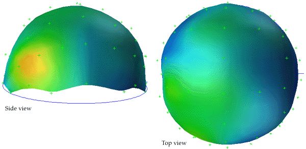
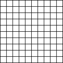
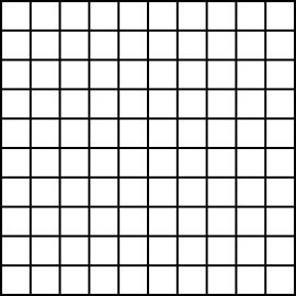
The following shows a planar projection from the hemisphere on the left and the same data with a stereographic projection. The compression near the rim is clearly reduced greatly improving the visibility of the results in that region.

Note that in the above, after the projection has been performed, the resulting disk is scaled by a factor of 0.5 in order to retain the same dimensions as the hemisphere.
Cylindrical projection
Also sometimes known as a cylindric projection.The general cylindrical projection is one where lines of latitude are projected to equally spaced parallel lines and lines of longitude are projected onto not necessarily equally spaced parallel lines. The diagram below illustrates the basic projection, a line is projected from the centre of the sphere through each point on the sphere until it intersects the cylinder.

The equations are quite straightforward, if the cylinder is unwrapped and the horizontal axis is x and the vertical axis is y (origin in the vertical center and on the left side horizontally) then:
x = constant * alphay = constant * tan(beta)
Mercator projection
A Mercator projection is similar in appearange to a cylindrical projection but has a different distortion in the spacing of the lines of longitude. Like the cylindrical projection north and south are always vertical and east and west are always horizontal. Also it cannot represent the poles because the mathematics have an infinity singularity there. This is one of the more common projections used in mapping the Earth onto a flat surface. There is not a single Mercator projection because one can choose the maximum value for the latitudes, a common convention is illustrated below.
 Spherical or Equirectangular projection |
Mercator projection |
The equations for longitude and latitude in terms of normalised image coordinates (x,y) (-1..1) are as follows.
latitude = atan(exp(-2 * pi * y))
The reverse mapping is
y = ln((1 + sin(latitude))/(1 - sin(latitude))) / (4 pi)
 |
Cylindrical projections in general have an increased vertical stretching as one moves towards either of the poles. Indeed, the poles themselves can't be represented (except at infinity). This stretching is reduced in the >ercator projection by the natural logarithm scaling.
Direct Polar, known as Spherical or Equirectangular Projection
While not strictly a projection, a common way of representing spherical surfaces in a rectangular form is to simply use the polar angles directly as the horizontal and vertical coordinates. Since longitude varies over 2 pi and latitude only over pi, such polar maps are normally presented in a 2:1 ratio of width to height. The most noticeable distortion in these maps is the horizontal stretching that occurs as one approaches the poles from the equator, this culminates in the poles (a single point) being stretched to the whole width of the map.
An example of such a map is given below for the Earth.
While such maps are rarely used in cartography, they are very popular in computer graphics since it is the standard way of texture mapping a sphere.....hence the popularity of maps of the Earth as shown above.
<pHammer-Aitoff map projection
Conversion to/from longitude/latitude
Written by Paul BourkeApril 2005
An Aitoff map projection (attributed to David Aitoff circa 1889) is a class of azimuthal projection, basically an azimuthal equidistant projection where the longitude values are doubled (squeezing 2pi into pi) and the resulting 2D map is stretched in the horizontal axis to form a 2:1 ellipse. In a normal azimuthal projection all distances are preserved from the tangent plane point, this is not the case for a Aitoff projection, except along the vertical and horizontal axis. A modification to the Aitoff projection is the Hammer-Aitoff projection which has the property of preserving equal area over the whole map.
Conversion from longitude/latitude to Hammer-Aitoff coordinates (x,y)Consider longitude to range between -pi and pi, latitude between -pi/2 and pi/2.
| z2 = 1 + cos(latitude) cos(longitude/2) x = cos(latitude) sin(longitude/2) / z y = sin(latitude) / z |
(x,y) are each normalised coordinates, -1 to 1.
Conversion of Hammer-Aitoff coordinates to longitude/latitude
| z2 = 1 - x2/2 - y2/2 longitude = 2 atan(sqrt(2) x z / (2 z2 - 1)) latitude = asin(sqrt(2) y z) |
The Hammer-Aitoff map is limited to where (x longitude) >= 0.
Example: Conversion of longitude/latitude to Hammer-Aitoff coordinates
Grid test pattern, eg: spherical panoramic map |
Resulting Hammer-Aitoff projection |
Example: Conversion of Hammer-Aitoff coordinates to longitude/latitude
 Cosmic microwave background |
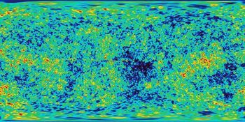 Spherical projection |
Transformations on the plane
Written by Paul BourkeJanuary 1987
The following describes the 2d transformation of a point on a plane
P = ( x , y ) -> P' = ( x' , y' )
Translation
A translation (shift) by T x in the x direction and T y in the y direction isx' = x + Tx
y' = y + Ty
Scaling
A scaling by S x in the x direction and S y in the y directions about the origin isx' = Sx x
y' = Sy y
If Sx and Sy are not equal this results in a stretching along the axis of the larger scale factor.
To scale about a particular point, first translate to the origin, scale, and translate back to the original position. For example, to scale about the point (x0,y0)
x' = x0 + Sx ( x - x0 )
y' = y0 + Sy ( y - y0 )
Rotation
Rotation about the origin by an angle A in a clockwise direction isx' = x cos(A) + y sin(A)
y' = y cos(A) - x sin(A)
To rotate about a particular point apply the same technique as described for scaling, translate the coordinate system to the origin, rotate, and the translate back.
Reflection
Reflection about the x axisx' = x
y' = - y
Reflection about the y axis
x' = - x
y' = y
Reflections about an arbitrary line involve possibly a translation so that a point on the line passes through the origin, a rotation of the line to align it with one of the axis, a reflection, inverse rotation and inverse translation.
Shear
A shear by SH x in the x axis is accomplished withx' = SHx x
y' = y
A shear by SHy in the y axis is accomplished with
x' = x
y' = SHy y
Coordinate System Transformation
Written by Paul BourkeJune 1996
There are three prevalant coordinate systems for describing geometry in 3 space, cartesian, cylindrical, and spherical (polar). They all provide a way of uniquely defining any point in 3D.
The following illustrates the three systems.

Equations for converting between cartesian and cylindrical coordinates

Equations for converting between cylindrical and spherical coordinates

Equations for converting between cartesian and spherical coordinates

Euler AnglesWritten by Paul BourkeJune 2000 Extaction of Euler angles from general rotation matrix |
 |
Rotations about each axis are often used to transform between different coordinate systems, for example, to direct the virtual camera in a flight simulator. These angles often go by different names, in the discussion here I will use a right hand coordinate system (y "forward", x to the right, and z upwards). As such rotation about the z axis will be referred to as direction, rotation about the y axis is roll (sometimes called bank), and rotation about the x axis is pitch. Further, a rotation will be considered positive if it is clockwise when looking down the axis towards the origin. Other conventions will be left as an exercise for the reader.
The three rotation matrices are given below, note that they seem asymmetric with respect to the sign of the sin() term.Rotation by tx about the x axis
|
= |
|
|
Rotation by ty about the y axis
|
= |
|
|
Rotation angle tz about the z axis
|
= |
|
|
A characteristic of applying these transformations is that the order is important. If the rotation matrices above are called Rx(t), Ry(t), and Rz(t) respectively then applying the rotations in the order Rz(t) Rx(t) Ry(t) will in general result in a different result to another order, say Rx(t) Ry(t) Rz(t). In what follows a particular order will be discussed and the other combinations will be left up to the reader to derive based on the same approach. The particular order of rotations applied here is to rotate about the y axis first (roll), they the x axis (pitch), then the z axis (direction). This is perhaps the most common order is usage in games and flight simulators.
|
= Rz(t) Rx(t) Ry(t) |
|
The single (combined) matrix is
|
One other requirement is given a new coordinate system how does one derive the corresponding three Euler angles. If the orthonormal vectors of the new coordinate system are X,Y,Z then the transformation matrix from (1,0,0), (0,1,0), (0,0,1) to the new coordinate system is
|
Y z = -sin(t x)
so
t x = asin(-Y z)
Also
so
t y = atan2(X z, Z z))
And lastly
so
t z = atan2(Y x, Y y)
Note:
-
The "programmers" function atan2() has been used above which uses the sign of the two arguments to calculate the correct quadrant of the result, this is in contrast to the mathematical tan() function.
-
While the above gives particular values for tx, ty, and tz there are a number of cases where the solution is not unique. That is, there are multiple combinations of Euler angles that will give the same coordinate transformation.
Converting between left and right hand coordinate systems
Written by Paul BourkeMay 2001
Computer based modelling and rendering software seem to be split evenly between whether they use a left hand or right hand coordinate system, for example OpenGL uses a right hand system and PovRay a left hand system. This document describes bow to convert model coordinates and/or camera attributes when transferring models from one package to another. Each system is shown below, the difference involves how the cross product is defined...using the so-called left or right hand rule.

Note that the exact orientation of the axes above is not relevant, y need not be "pointing up", z need not be pointing "into the page". All axes orientations are equivalent to one of the above after a suitable rotation.
There are two ways to convert models between systems so that the rendered results are identical. The first involves inverting the x value (any single axes will do) of all vertices in the model and camera settings, the second uses the model and camera coordinates without change but requires a flipping of any rendered image horizontally. In what follows, the symbols p, d, and u will represent the vectors position, view direction, and up vector respectively.
Method 1 - inverting the x coordinates
Method 2 - flipping image horizontally
In this case the coordinates of the model and camera are used unchanged when transferring from one system to the other. As can be seen in the example below, the image ends up being horizontally flipped.
This is usually the preferred method, perhaps mainly because it avoids worrying about which system one is using until the end of the process, the image flipping can be built into post processing image tools. Also, it means that if one makes a mistake regarding which system is being using it doesn't affect the rendered result nearly as seriously than if one got made a mistake in the first method.
You may wonder why it is the horizontal axis that is flipped, what is so special about it? That arises because the flip is actually about the up vector which is traditionally vertical on the rendered image.
Classification of 3D to 2D projections
Written by Paul BourkeDecember 1994
The following classifies the most common projections used to represent 3D geometry on a 2D surface. Each projection type has a brief comment describing its unique characteristic.

Oblique projections
| An oblique projection is a parallel projection where the projecting lines are not perpendicular to the projection plane. The precise projection is defined by two anglesTwo common projections are:
|
 |
| For either one of the above projections values of most commonly employed are 45 degrees and 30 degrees. Coordinate transformations for a general oblique projection are |
 |
Note:
-
The first two transformations for xp and yp are all that is required to derive the transformation from 3D onto the 2D projection plane. The third trivial) transformation for z illustrates how an oblique projection is equivalent to a z axis shear followed by a parallel orthographic projection onto a x-y projection plane.
-
The x and y coordinate values within each z plane are shifted by an amount proportional to the z value of the plane. (ie: cos() / tan(
 )) so angles, distances, and parallel lines in any z plane are projected accurately, without distortion.
| Cavalier projection = 45 |  |
| Cavalier projection = 30 |  |
| Cabinet projection = 45 |  |
| Cabinet projection = 30 |  |
Correction of Planar (Stretch) Distortion
Written by Paul BourkeNovember 1989
The following mathematics and illustrations came from a project to undistort photographs taken of a flat piece of land. The photographs were taken from various angles to the ground and thus needed to be "straightened" so that relative area measures could be taken. The same technique could of course be used to intentionally distort rectangular areas.
The conventional (cartesian) method of uniquely specifying a point in 2 dimensions is by two coordinates. For the unit square below these two coordinates will be called mu and delta, they are the relative distances along the horizontal and vertical edges of the square.

If the square above is linearly distorted (stretched) the internal coordinate mesh is also distorted but the relative distances (mu and delta) of a point P along two connected edges remains the same.

To undistort any point P within the polygon we need to find the ratios mu and delta. Point A is given by:
Point B is given by
For the point P along the line AB
Substituting for A and B, equation 1
This gives two equations, one for the x coordinate and the other for the y coordinate, equation 2,3
Dividing equation (2) by (3) removes delta, solving for mu gives a quadratic of the form
where
After solving the quadratic for mu, delta can be calculated from (1) above.
Anamorphic ProjectionsWritten by Paul BourkeJanuary 1991 Source: glues.h and glues.c. Anamorphism is a Macintosh utility which takes a line drawing as a PICT file and performs various nonlinear distortions upon it. The distortions available have been chosen from those which have been used historically by artists (and forgers). |
 |
Each of the different distortions will be illustrated by using the following simple diagram.
For the following examples an additional grid will be placed over the image to further illustrate the nature of the distortion. Each type of distortion has controls associated with it, these are indicated by black "blobs" at the current position of the control points. To vary these parameters simply click and drag the control points.
| Cylindrical |  |
| Conical |
| Spherical |  |
| Parabolic |
| Rectonical |  |
Notes
-
The only PICT drawing primitives which can be used are line segments.
-
Since the distortions are non linear, the distorted points alone a line segment do not lie in a straight line between the distorted end points of the line segment. Thus each line is split into a number of line segments in order to approximate the generally curved nature of the distorted lines. The result of this is distorted drawings with a much larger number of line segments.

Mappings in the Complex Plane
Written by Paul BourkeJuly 1997
The following illustrates the general form of various mappings in the complex plane. The mappings are applied to part of a unit disk centered at the origin as shown on the left hand side. The circle is filled with rays from the origin and arcs centered about the origin. A series of coloured rays further illustrate the mapping orientation.
z |
exp(z) |
z |
log(z) |
z |
sqrt(z) |
z |
asin(z) |
z |
acos(z) |
z |
atan(z) |
z |
sin(z) |
z |
cos(z) |
z |
tan(z) |
z |
sinh(z) |
z |
cosh(z) |
z |
tanh(z) |
z |
z2 |
z |
z2 + z |
z |
1 / (z + 1) |
z |
(z - 1) / (z + 1) |

z |
(z2 - 1) / (z2 + 1) |

z |
(z - a) / (z + b) |

z |
(z2 + z - 1) / (z2 + z + 1) |

z |
(z2 + z + 1) / (z + 1) |

World to Screen Projection Transformation
Written by Paul BourkeDecember 1994
The representation by computer of 3 dimensional forms is normally restricted to the projection onto a plane, namely the 2 dimensional computer screen or hardcopy device. The following is a procedure that transforms points in 3 dimensional space to screen coordinates given a particular coordinate system, camera and projection plane models. This discussion describes the mathematics required for a perspective projection including clipping to the projection pyramid with a front and back cutting plane. It assumes the projection plane to be perpendicular to the view direction vector and thus it does not allow for oblique projections.
Included in the appendices is source code (written in the C programming language) implementing all the processes described.
Coordinate systemIn what follows a so called right handed coordinate system is used, it has the positive x axis to the right, the positive z axis upward, and the positive y axis forward (into the screen or page).
Conversion between this and other coordinate systems simply involves the swapping and/or negation of the appropriate coordinates.
Camera modelThe camera is fundamentally defined by its position (from), a point along the positive view direction vector (to), a vector defining "up" (up), and a horizontal and vertical aperture (angleh, anglev).
These parameters are illustrated in the following figure.
One obvious restriction is that the view direction must not be collinear with the up vector. In practical implementations, including the one given in the appendices, the up vector need not be a unit vector.
Other somewhat artificial variables in the camera model used here are front and back clipping planes, a perspective/oblique projection flag, and a multiplicative zoom factor. The clipping planes are defined as positive distances along the view direction vector, in other words they are perpendicular to the view direction vector. As expected all geometry before the front plane and beyond the back plane is not visible. All geometry which crosses these planes is clipped to the appropriate plane. Thus geometry visible to a camera as described here lies within a truncated pyramid.
Screen model
The projection plane (computer screen or hardcopy device) can be defined in many ways. Here the central point, width and height are used. The following will further assume the unfortunate convention, common in computer graphics practice, that the positive vertical axis is downward. The coordinates of the projection space will be referred to as (h,v).

Note that normally in computer windowing systems the window area is defined as an rectangle between two points (left,top) and (right,bottom). Transforming this description into the definition used here is trivial, namely
horizontal center = (left + right) / 2vertical center = (top + bottom) / 2
width = right - left
height = bottom - top
The units need not be specified although they are generally pixel's, it is assumed that there are drawing routines in the same units. It is also assumed that the computer screen has a 1:1 aspect ratio, a least as far as the drawing routines are concerned.
A relationship could be made between the ratio of the horizontal and vertical camera aperture and the horizontal and vertical ratio of the display area. Here it will be assumed that the display area (eg: window) has the same proportions as the ratio of the camera aperture. In practice this simply means that when the camera aperture is modified, the window size is also modified so as to retain the correct proportions.
AlgorithmThe procedure for determining where a 3D point in world coordinates would appear on the screen is as follows:

Transforming a line segment involves determining which piece, if any, of the line segment intersects the view volume. The logic is shown below.

Clipping
Two separate clipping processes occur. The first is clipping to the front and back clipping planes and is done after transforming to eye coordinates. The second is clipping to the view pyramid and is performed after transforming to normalised coordinates at which point it is necessary to clip 2D line segments to a square centered at the origin of length and height of 2.
Source code
transform.c, transform.h.
Cubic to Cylindrical conversion
Written by Paul BourkeNovember 2003, Updated may 2006
The following discusses the transformation of a cubic environment map (90 degree perspective projections onto the face of a cube) into a cylindrical panoramic image. The driver for this was the creation of cylindrical panoramic images from rendering software that didn't explicitly support panoramic creation. The software was scripted to create the 6 cubic images and this utility created the panoramic.
UsageUsage: cube2cyl [options] filemask filemask can contain %c which will substituted with each of [l,r,t,d,b,f] For example: "blah_%c.tga" or "%c_something.tga" Options -a n sets antialiasing level, default = 2 -v n vertical aperture, default = 90 -w n sets the output image width, default = 3 * cube image width -c enable top and bottom cap texture generation, default = off -s split cylinder into 4 pieces, default = offFile name conventions
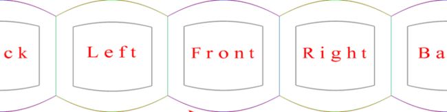
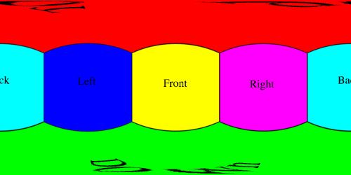
The names of the cubic maps are assumed to contain the letters 'f', 'l', 'r', 't', 'b', 'd' that indicate the face (front,left,right,top,back,down). The file mask needs to contain "%c" which specifies the view.
So for example the following cubic maps would be specified as %c_starmap.tga,
l_starmap.tga, r_starmap.tga, f_starmap.tga,
t_starmap.tga, b_starmap.tga, d_starmap.tga.
Note the orientation convention for the cube faces.
cube2cyl -a 3 -v 90
Note that in this special case the top of the face should coincide with the top of the cylindrical panoramic.
cube2cyl -a 3 -v 120

cube2cyl -a 3 -v 150

Geometry
The mapping for each pixel in the destination cylindrical panoramic from the correct location on the appropriate cubic face is relatively straightforward. The horizontal axis maps linearly onto the angle about the cylinder. The vertical axis of the panoramic image maps onto the vertical axis of the cylinder by a tan relationship.
In particular, if (i,j) is the pixel index of the panoramic normalised to (-1,+1) the the direction vector is given as follows.y = j tan(v/2)
z = sin(i pi)


This direction vector is then used within the texture mapped cubic geometry. The face of the cube it intersects needs to be found and then the pixel the ray passes through is determined (intersection of the direction vector with the plane of the face). Critical to obtaining good quality results is antialiasing, in this implementation a straightforward constant weighted supersampling is used.
Example 1Cubic map
Cylindrical panoramic (90 degrees)
Example 2
Cubic map

Cylindrical panoramic (90 degrees)

Notes
- The vertical aperture must be greater than 0 and less than 180 degrees. The current implementation limits it to be between 1 and 179 degrees.
- While not a requirement, the current implementation retains the height to width ratio of the output image to the same as the vertical aperture to horizontal aperture.
- Typically antialiasing levels of 3 are more than enough.
One can equally form the image textures for a top and bottom cap. The following is an example of such caps, in this case the vertical field of view is 90 degrees so the cylinder is cubic (diameter of 2 and height of 2 units). It should be noted that a relatively high degree of tessellation is required for the cylindrical mesh if the linear approximations of the edges is not to create seam artifacts.
 |
 |
 |
The aspect of the cylinder height to the width for an undistorted cylindrical vies and for the two caps to match is tan(verticalFOV/2).
Converting to and from 6 cubic environment maps and a spherical map
Written by Paul BourkeFebruary 2002, updated May 2006 Introduction
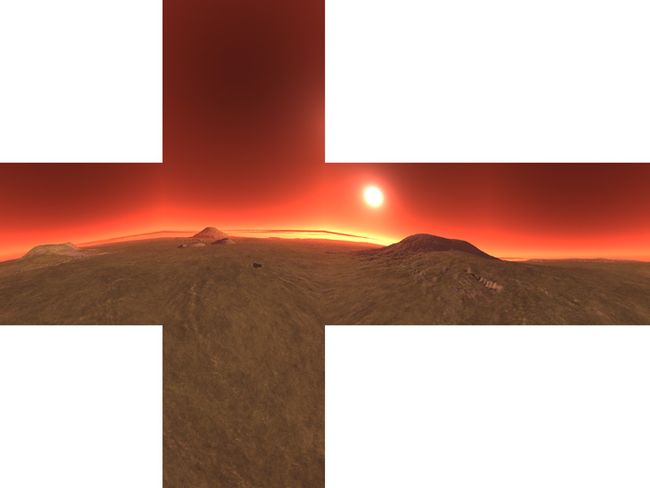
There are two common methods of representing environment maps, cubic and spherical. In cubic maps the virtual camera is surrounded by a cube the 6 faces of which have an appropriate texture map. These texture maps are often created by imaging the scene with six 90 degree fov cameras giving a left, front, right, back, top, and bottom texture. In a spherical map the camera is surrounded by a sphere with a single spherically distorted texture. This document describes bow to convert 6 cubic maps into a single spherical map.
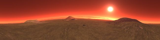
ExampleAs an illustrative example the following 6 images are the textures placed on the cubic environment, they are arranged as an unfolded cube. Below that is the spherical texture map that would give the same appearance if applied as a texture to a sphere about the camera.
 |
Maps courtesy of Ben Syverson |

The conversion process involves two main stages. The goal is to determine the best estimate of the colour at each pixel in the final spherical image given the 6 cubic texture images. The first stage is to calculate the polar coordinates corresponding to each pixel in the spherical image. The second stage is to use the polar coordinates to form a vector and find which face and which pixel on that face the vector (ray) strikes. In reality this process is repeated a number of times at slightly different positions in each pixel in the spherical image and an average is used in order to avoid aliasing effects.
If the coordinates of the spherical image are (i,j) and the image has width "w" and height "h" then the normalised coordinates (x,y) each ranging from -1 to 1 are given by:
| x = 2 i / w - 1 y = 2 j / h - 1 or y = 1 - 2 j / h depending on the position of pixel 0 |
The polar coordinates theta and phi are derived from the normalised coordinates (x,y) below. theta ranges from 0 to 2 pi and phi ranges from -pi/2 (south pole) to pi/2 (north pole). Note there are two vertical relationships in common use, linear and spherical. In the former phi is linearly related to y, in the later there is a sine relationship.
| theta = x pi phi = y pi / 2 or phi = asin(y) for spherical vertical distortion |
The polar coordinates (theta,phi) are turned into a unit vector (view ray from the camera) as below. This assumes a right hand coordinate system, x to the right, y upwards, and z out of the page. The front view of the cubic map is looking from the origin along the positive z axis.
| x = cos(phi) cos(theta) y = sin(phi) z = cos(phi) sin(theta) |
The intersection of this ray is now found with the faces of the cube. Once the intersection point is found the coordinate on the square face specifies the corresponding pixel and therefore colour associated with the ray.
Mapping geometry |
 |
 |
 |
 |

 |
|||
 |
 |
 |
|
Usage: cube2sphere [options] filemask
filemask should contain %c which will substituted with each of [l,r,t,d,b,f]
For example: "blah_%c.tga" or "%c_something.tga"
Options
   -w n     sets the output image width, default = 4*inwidth
  -w1 n     sub image position 1, default: 0
  -w2 n     sub image position 2, default: width
   -h n     sets the output image height, default = width/2
   -a n     sets antialiasing level, default = 1 (none)
   -s       use sine correction for vertical axis
 |
|||
 |
 |
||
 |
Convert spherical projections to cylindrical projection
Written by Paul BourkeFebruary 2010
The following utility was written to convert spherical projections into cylindrical projections. Of course only a slice of the spherical projection is used. The original reason for developing this was to convert video content from the LadyBug-3 camera (spherical projection) to a suitable image for a 360 cylindrical display. This a command line utility and as such straightforward to script to convert sequences of frames that make up a movie.
sph2pan [options] sphericalimagename
Options:
-t n       set max theta on vertical axis of panoramic, 0...90 (default: 45)
-a n       set antialias level, 1 upwards, 2 or 3 typical (default: 2)
-w n       width of the spherical image
-r n       horizontal rotation angle (default: 0)
-v n       vertical rotation angle (default: 0)
-f         flip insideout (default: off)
Sample spherical projection (from the LadyBug-3)
Click for original image (5400x2700 pixels).
As with all such image transformations, one considers a point in the destination image noting that the pont may be a sub pixel (required for supersampling antialiasing). This point corresponds to a vector in 3D space, this is then used to determine the corresponding point in the input image. Options such as rotations and flips correspond to operations on the 3D vector.
Sample derived cylindrical projectionsThe following show example transformations illustrating some of the more important options. In particular the ability to specify the vertical field of view and the vertical offset for the cylindrical image.

sph2pan -w 800 -v -7.5 dervish_sph.tga

sph2pan -w 800 -v -7.5 -t 60 dervish_sph.tga

sph2pan -w 800 -v -7.5 -t 60 -r 90 dervish_sph.tga
From: http://paulbourke.net/geometry/transformationprojection/