【Keras-DenseNet】CIFAR-10

系列连载目录

• 请查看博客 《Paper》 4.1 小节 【Keras】Classification in CIFAR-10 系列连载

学习借鉴

• github：BIGBALLON/cifar-10-cnn
• 知乎专栏：写给妹子的深度学习教程

参考

• 本地远程访问Ubuntu16.04.3服务器上的TensorBoard
• 《Densely Connected Convolutional Networks》

代码

• 链接：https://pan.baidu.com/s/1nWcfuzH_Cv-yewkYwZJP0w
  提取码：pvst

硬件

• TITAN XP

---

1 DenseNet

论文解读【DenseNet】《Densely Connected Convolutional Networks》

结构如下

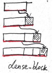
2 DenseNet-100x12

其实不看代码之前，有点被第一节那个 $n\ast (n-1)/2$ 图带偏了，其实代码如下面的图这个样子（不断堆叠），本质是一样，不过得仔细琢磨下。

代码：Caffe 版
Caffe 代码可视化工具

我们用 keras 实现，总框架和 【Keras-ResNet】CIFAR-10 一样

1）导入库，设置好超参数

import keras
import numpy as np
import math
from keras.datasets import cifar10
from keras.preprocessing.image import ImageDataGenerator
from keras.models import Model
from keras.initializers import he_normal
from keras.layers import Dense, Input, add, Activation, Lambda, concatenate
from keras.layers import Conv2D, AveragePooling2D, GlobalAveragePooling2D
from keras.layers.normalization import BatchNormalization
from keras.layers.merge import Concatenate
from keras import optimizers, regularizers
from keras.callbacks import LearningRateScheduler, TensorBoard

growth_rate        = 12 
depth              = 100
compression        = 0.5

img_rows, img_cols = 32, 32
img_channels       = 3
num_classes        = 10
batch_size         = 64         # 64 or 32 or other
epochs             = 300
iterations         = 782       
weight_decay       = 1e-4

log_filepath  = './densenet_100'

2）数据预处理并设置 learning schedule

def color_preprocessing(x_train,x_test):
    x_train = x_train.astype('float32')
    x_test = x_test.astype('float32')
    mean = [125.307, 122.95, 113.865]
    std  = [62.9932, 62.0887, 66.7048]
    for i in range(3):
        x_train[:,:,:,i] = (x_train[:,:,:,i] - mean[i]) / std[i]
        x_test[:,:,:,i] = (x_test[:,:,:,i] - mean[i]) / std[i]
    return x_train, x_test

def scheduler(epoch):
    if epoch < 150:
        return 0.1
    if epoch < 225:
        return 0.01
    return 0.001

# load data
(x_train, y_train), (x_test, y_test) = cifar10.load_data()
y_train = keras.utils.to_categorical(y_train, num_classes)
y_test  = keras.utils.to_categorical(y_test, num_classes)
x_train, x_test = color_preprocessing(x_train, x_test)

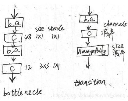
3）定义网络结构

如上图所示，dense_block 中的箭头就是 bottleneck 层，下面的代码中，dense_block concatenate 了16次， dense_block 后接一个transition 来 compress channels.

def conv(x, out_filters, k_size):
    return Conv2D(filters=out_filters,
                  kernel_size=k_size,
                  strides=(1,1),
                  padding='same',
                  kernel_initializer='he_normal',
                  kernel_regularizer=regularizers.l2(weight_decay),
                  use_bias=False)(x)

def dense_layer(x):
    return Dense(units=10,
                 activation='softmax',
                 kernel_initializer='he_normal',
                 kernel_regularizer=regularizers.l2(weight_decay))(x)

def bn_relu(x):
    x = BatchNormalization(momentum=0.9, epsilon=1e-5)(x)
    x = Activation('relu')(x)
    return x

def bottleneck(x):
    channels = growth_rate * 4
    x = bn_relu(x)
    x = conv(x, channels, (1,1)) # 48
    x = bn_relu(x)
    x = conv(x, growth_rate, (3,3)) # 12
    return x

# feature map size and channels half
def transition(x, inchannels):
    outchannels = int(inchannels * compression)
    x = bn_relu(x)
    x = conv(x, outchannels, (1,1))
    x = AveragePooling2D((2,2), strides=(2, 2))(x)
    return x, outchannels

def dense_block(x,blocks,nchannels):
    concat = x
    for i in range(blocks):
        x = bottleneck(concat)
        concat = concatenate([x,concat], axis=-1)
        nchannels += growth_rate
    return concat, nchannels

4）搭建网络
每个 bottleneck 结构有 2 层（channels 分别为 growth_rate*4 和 growth_rate），每个 dense_block 有16个bottleneck 也就是 32层，每个 transition 有 1 层（channels 减半），按照如下代码的结构设计，总层数 = conv1 + 32 + 1 + 32 + 1 + 32 + fc = 96+4 = 100

def densenet(img_input,classes_num):
    nblocks = (depth - 4) // 6 # 16
    nchannels = growth_rate * 2 # 12*2 = 24

    x = conv(img_input, nchannels, (3,3)) # 32*32*3 to 32*32*24
    # 32*32*24 to 32*32*(24+nblocks*growth_rate) = 24+16*12 = 216
    x, nchannels = dense_block(x,nblocks,nchannels) # 32*32*24 to 32*32*216
    x, nchannels = transition(x,nchannels) # 32*32*216 to 16*16*108
    
    x, nchannels = dense_block(x,nblocks,nchannels) # 16*16*108 to 16*16*（108+16*12） = 16*16*300
    x, nchannels = transition(x,nchannels) # 16*16*300 to 8*8*150
    
    x, nchannels = dense_block(x,nblocks,nchannels) # 8*8*150 to 8*8*(150+16*12) = 8*8*342
    x = bn_relu(x)
    x = GlobalAveragePooling2D()(x) #8*8*342 to 342
    x = dense_layer(x) # 342 to 10
    return x

5）生成模型

# build network
img_input = Input(shape=(img_rows,img_cols,img_channels))
output    = densenet(img_input,10)
model     = Model(img_input, output)
print(model.summary())

6）开始训练

# set optimizer
sgd = optimizers.SGD(lr=.1, momentum=0.9, nesterov=True)
model.compile(loss='categorical_crossentropy', optimizer=sgd, metrics=['accuracy'])

# set callback
tb_cb = TensorBoard(log_dir=log_filepath, histogram_freq=0)
change_lr = LearningRateScheduler(scheduler)
cbks = [change_lr,tb_cb]

# set data augmentation
datagen = ImageDataGenerator(horizontal_flip=True,
                             width_shift_range=0.125,
                             height_shift_range=0.125,
                             fill_mode='constant',cval=0.)
datagen.fit(x_train)

# start training
model.fit_generator(datagen.flow(x_train, y_train,batch_size=batch_size), 
                    steps_per_epoch=iterations, 
                    epochs=epochs, 
                    callbacks=cbks,
                    validation_data=(x_test, y_test))
model.save('densenet_100x24.h5')

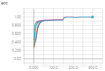
7）结果分析
training accuracy 和 training loss


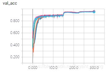
test accuracy 和 test loss

同 epoch 下的结果

最终的结果

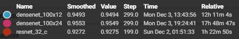
不得不佩服 DenseNet，是真的猛

8）parameters 和 model size

• resnet_32_c
  Total params: 470,410
  Trainable params: 468,042
  Non-trainable params: 2,368

• densenet_100×12
  Total params: 793,150
  Trainable params: 769,162
  Non-trainable params: 23,988

• densenet_100×24
  修改 growth_rate = 24
  修改 log_filepath = './densenet_100x24'
  修改 model.save('densenet_100x24.h5'),其它不变
  Total params: 3,068,482
  Trainable params: 3,020,506
  Non-trainable params: 47,976

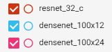
模型大小（model size）

resnet_32_c 的大小为 3.93M

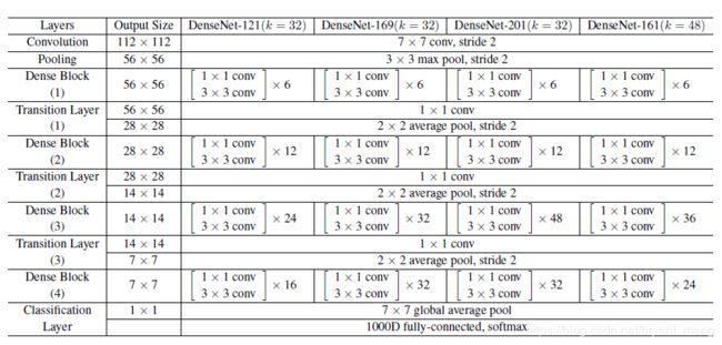
3 densenet 各种版本

前两层的 convolution 和 pooling 用一个 convolution（channels 等于两倍的 growth_rate）代替，后面结构完全和论文中的结构设计一样。

3.1 densenet_121×32

修改 growth_rate = 32
修改 log_filepath = './densenet_121×32'
修改 model.save('densenet_121×32.h5')
修改网络结构如下，其它不改变

def densenet(img_input,classes_num):
    nchannels = growth_rate * 2
    x = conv(img_input, nchannels, (3,3)) 

    x, nchannels = dense_block(x,6,nchannels) 
    x, nchannels = transition(x,nchannels) 
    
    x, nchannels = dense_block(x,12,nchannels) 
    x, nchannels = transition(x,nchannels)
    
    x, nchannels = dense_block(x,24,nchannels) 
    x, nchannels = transition(x,nchannels)
    
    x, nchannels = dense_block(x,16,nchannels) 
    
    x = bn_relu(x)
    x = GlobalAveragePooling2D()(x)
    x = dense_layer(x) # 342 to 10
    return x

Total params: 7,039,818
Trainable params: 6,956,298
Non-trainable params: 83,520

3.2 densenet_169×32

修改 growth_rate = 32
修改 log_filepath = './densenet_169×32'
修改 model.save('densenet_169×32.h5')
修改网络结构如下，其它不改变

def densenet(img_input,classes_num):
    nchannels = growth_rate * 2
    x = conv(img_input, nchannels, (3,3)) 

    x, nchannels = dense_block(x,6,nchannels) 
    x, nchannels = transition(x,nchannels) 
    
    x, nchannels = dense_block(x,12,nchannels) 
    x, nchannels = transition(x,nchannels)
    
    x, nchannels = dense_block(x,32,nchannels) 
    x, nchannels = transition(x,nchannels)
    
    x, nchannels = dense_block(x,32,nchannels) 
    
    x = bn_relu(x)
    x = GlobalAveragePooling2D()(x)
    x = dense_layer(x)
    return x

Total params: 12,651,594
Trainable params: 12,493,322
Non-trainable params: 158,272

3.3 densenet_201×32

修改 growth_rate = 32
修改 log_filepath = './densenet_201×32'
修改 model.save('densenet_201×32.h5')
修改网络结构如下，其它不改变

def densenet(img_input,classes_num):
    nchannels = growth_rate * 2
    x = conv(img_input, nchannels, (3,3)) 

    x, nchannels = dense_block(x,6,nchannels) 
    x, nchannels = transition(x,nchannels) 
    
    x, nchannels = dense_block(x,12,nchannels) 
    x, nchannels = transition(x,nchannels)
    
    x, nchannels = dense_block(x,48,nchannels) 
    x, nchannels = transition(x,nchannels)
    
    x, nchannels = dense_block(x,32,nchannels) 
    
    x = bn_relu(x)
    x = GlobalAveragePooling2D()(x)
    x = dense_layer(x)
    return x

Total params: 18,333,258
Trainable params: 18,104,330
Non-trainable params: 228,928

3.4 densenet_161×48

修改 growth_rate = 48
修改 log_filepath = './densenet_161×48'
修改 model.save('densenet_161×48.h5')
修改网络结构如下，其它不改变

def densenet(img_input,classes_num):
    nchannels = growth_rate * 2
    x = conv(img_input, nchannels, (3,3)) 

    x, nchannels = dense_block(x,6,nchannels) 
    x, nchannels = transition(x,nchannels) 
    
    x, nchannels = dense_block(x,12,nchannels) 
    x, nchannels = transition(x,nchannels)
    
    x, nchannels = dense_block(x,36,nchannels) 
    x, nchannels = transition(x,nchannels)
    
    x, nchannels = dense_block(x,24,nchannels) 
    
    x = bn_relu(x)
    x = GlobalAveragePooling2D()(x)
    x = dense_layer(x)
    return x

Total params: 26,702,122
Trainable params: 26,482,378
Non-trainable params: 219,744

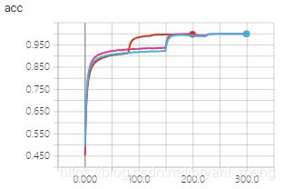
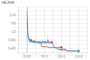
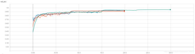
3.5 结果比较

• training accuracy and loss
  
  
• testing accuracy and loss
  
  放大一点看看
  
  
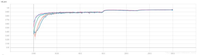
  结合时间和精度来说，densenet_121×32性价比最高，其精度最好，时间相对最小模型densenet_100×12也还不错。

3.6 模型大小

4 总结

• DenseNet 的第一个卷积的 channels 为 growth_rate×2
• dense_block 中每个bottleneck，有两个卷积，第一个卷积的 channels 为 growth_rate×4，第二个卷积的 channels 为 growth_rate

5 系列连载

• 【Keras-LeNet】CIFAR-10
• 【Keras-NIN】CIFAR-10
• 【Keras-VGG】CIFAR-10
• 【Keras-ResNet】CIFAR-10
• 【Keras-DenseNet】CIFAR-10