Basic Statistics
Quartile calculator Q1, Q3
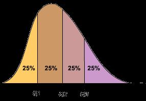
In statistics, a quartile, a type of quantile, is three points that divide sorted data set into four equal groups (by count of numbers), each representing a fourth of the distributed sampled population.
There are three quartiles: the first quartile (Q1), the second quartile (Q2), and the third quartile (Q3).
The first quartile (lower quartile, QL), is equal to the 25th percentile of the data. (splits off the lowest 25% of data from the highest 75%)
The second (middle) quartile or median of a data set is equal to the 50th percentile of the data (cuts data in half)
The third quartile, called upper quartile (QU), is equal to the 75th percentile of the data. (splits off the lowest 75% of data from highest 25%)
How we calculating quartiles?
We sort set of data with n items (numbers) and pick n/4-th item as Q1, n/2-th item as Q2 and 3n/4-th item as Q3 quartile. If indexes n/4, n/2 or 3n/4 aren't integers then we use interpolation between nearest items.
For example, for n=100 items, the first quartile Q1 is 25th item of ordered data, quartile Q2 is 50th item and quartile Q3 is 75th item. Zero quartile Q0 would be minimal item and the fourth quartile Q4 would be the maximum item of data, but these extreme quartiles are called minimum resp. maximum of set.
IQR
四分位距(interquartile range, IQR)。是描述统计学中的一种方法,以确定第三四分位数和第一四分位数的分别(即 $Q_{1}/Q_{3}$的差距)[1]。与方差、标准差一样,表示统计资料中各变量分散情形,但四分差更多为一种稳健统计(robust statistic)。
四分位差(Quartile Deviation, QD),是 $Q_{1},Q_{3}$ 的差距,即$QD=(Q_{3}-Q_{1})/2$ 。
Outlier
In statistics, an outlier is an observation point that is distant from other observations. An outlier may be due to variability in the measurement or it may indicate experimental error; the latter are sometimes excluded from the data set.
Outliers can occur by chance in any distribution, but they often indicate either measurement error or that the population has a heavy-tailed distribution.
Define Outlier
Outlier> $Q_{1}-1.5(IQR)$$ 或 <$$Q_{3}+1.5(IQR)$ # Box Plot
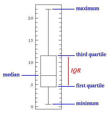
In descriptive statistics, a box plot or boxplot is a convenient way of graphically depicting groups of numerical data through their quartiles. Box plots may also have lines extending vertically from the boxes (whiskers) indicating variability outside the upper and lower quartiles, hence the terms box-and-whisker plot and box-and-whisker diagram. Outliers may be plotted as individual points.
This simplest possible box plot displays the full range of variation (from min to max), the likely range of variation (the IQR), and a typical value (the median). Not uncommonly real datasets will display surprisingly high maximums or surprisingly low minimums called outliers. John Tukey has provided a precise definition for two types of outliers:
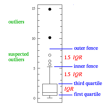
Outliers are either 3×IQR or more above the third quartile or 3×IQR or more below the first quartile.
Suspected outliers are are slightly more central versions of outliers: either 1.5×IQR or more above the third quartile or 1.5×IQR or more below the first quartile.
If either type of outlier is present the whisker on the appropriate side is taken to 1.5×IQR from the quartile (the "inner fence") rather than the max or min, and individual outlying data points are displayed as unfilled circles (for suspected outliers) or filled circles (for outliers). (The "outer fence" is 3×IQR from the quartile.)
If the data happens to be normally distributed,
IQR = 1.35 σ
where σ is the population standard deviation.
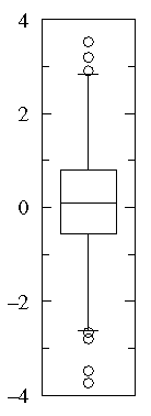
Suspected outliers are not uncommon in large normally distributed datasets (say more than 100 data-points). Outliers are expected in normally distributed datasets with more than about 10,000 data-points. Here is an example of 1000 normally distributed data displayed as a box plot:
Note that outliers are not necessarily "bad" data-points; indeed they may well be the most important, most information rich, part of the dataset. Under no circumstances should they be automatically removed from the dataset. Outliers may deserve special consideration: they may be the key to the phenomenon under study or the result of human blunders.
Numpy and Pandas Tutorials
The following code is to help you play with Numpy, which is a library
that provides functions that are especially useful when you have to
work with large arrays and matrices of numeric data, like doing
matrix matrix multiplications. Also, Numpy is battle tested and
optimized so that it runs fast, much faster than if you were working
with Python lists directly.
The array object class is the foundation of Numpy, and Numpy arrays are like
lists in Python, except that every thing inside an array must be of the
same type, like int or float.
import numpy as np

#To see Numpy arrays in action

array = np.array([1, 4, 5, 8], float)
print (array)
print ("")
array = np.array([[1, 2, 3], [4, 5, 6]], float)  # a 2D array/Matrix
print (array)
[ 1. 4. 5. 8.]
[[ 1. 2. 3.]
[ 4. 5. 6.]]## You can index, slice, and manipulate a Numpy array much like you would with a
#a Python list.
# To see array indexing and slicing in action
array = np.array([1, 4, 5, 8], float)
print (array)
print ("")
print (array[1])
print ("")
print (array[:2])
print ("")
array[1] = 5.0
print (array[1])[ 1. 4. 5. 8.]
4.0
[ 1. 4.]
5.0# To see Matrix indexing and slicing in action
two_D_array = np.array([[1, 2, 3], [4, 5, 6]], float)
print (two_D_array)
print ("")
print (two_D_array[1][1])
print ("")
print (two_D_array[1, :])
print ("")
print (two_D_array[:, 2])[[ 1. 2. 3.]
[ 4. 5. 6.]]
5.0
[ 4. 5. 6.]
[ 3. 6.]# Change False to True to see Array arithmetics in action
array_1 = np.array([1, 2, 3], float)
array_2 = np.array([5, 2, 6], float)
print (array_1 + array_2)
print ("")
print (array_1 - array_2)
print ("")
print (array_1 * array_2)[ 6. 4. 9.]
[-4. 0. -3.]
[ 5. 4. 18.]# Change False to True to see Matrix arithmetics in action
array_1 = np.array([[1, 2], [3, 4]], float)
array_2 = np.array([[5, 6], [7, 8]], float)
print (array_1 + array_2)
print ("")
print (array_1 - array_2)
print ("")
print (array_1 * array_2)[[ 6. 8.]
[ 10. 12.]]
[[-4. -4.]
[-4. -4.]]
[[ 5. 12.]
[ 21. 32.]]#In addition to the standard arthimetic operations, Numpy also has a range of
#other mathematical operations that you can apply to Numpy arrays, such as
#mean and dot product.
#Both of these functions will be useful in later programming quizzes.
array_1 = np.array([1, 2, 3], float)
array_2 = np.array([[6], [7], [8]], float)
print (np.mean(array_1))
print (np.mean(array_2))
print ("")
print (np.dot(array_1, array_2))2.0
7.0
[ 44.]
Pandasimport pandas as pd
The following code is to help you play with the concept of Series in Pandas.
You can think of Series as an one-dimensional object that is similar to
an array, list, or column in a database. By default, it will assign an
index label to each item in the Series ranging from 0 to N, where N is
the number of items in the Series minus one.
Please feel free to play around with the concept of Series and see what it does
*This playground is inspired by Greg Reda's post on Intro to Pandas Data Structures:
http://www.gregreda.com/2013/...
# To create a Series object

series = pd.Series(['Dave', 'Cheng-Han', 'Udacity', 42, -1789710578])
print (series)
0 Dave
1 Cheng-Han
2 Udacity
3 42
4 -1789710578
dtype: object
You can also manually assign indices to the items in the Series when
creating the series
# Change False to True to see custom index in action

series = pd.Series(['Dave', 'Cheng-Han', 359, 9001],
                   index=['Instructor', 'Curriculum Manager',
                          'Course Number', 'Power Level'])
print (series)
Instructor Dave
Curriculum Manager Cheng-Han
Course Number 359
Power Level 9001
dtype: object
You can use index to select specific items from the Series
series = pd.Series(['Dave', 'Cheng-Han', 359, 9001],
                   index=['Instructor', 'Curriculum Manager',
                          'Course Number', 'Power Level'])
print series['Instructor']
print ""
print series[['Instructor', 'Curriculum Manager', 'Course Number']]
Dave
Instructor Dave
Curriculum Manager Cheng-Han
Course Number 359
dtype: object
You can also use boolean operators to select specific items from the Series
cuteness = pd.Series([1, 2, 3, 4, 5], index=['Cockroach', 'Fish', 'Mini Pig',
                                             'Puppy', 'Kitten'])
print (cuteness > 3)
print ("")
print (cuteness[cuteness > 3])
Cockroach False
Fish False
Mini Pig False
Puppy True
Kitten True
dtype: bool
Puppy 4
Kitten 5
dtype: int64
Dataframe
import numpy as np
import pandas as pd
The following code is to help you play with the concept of Dataframe in Pandas.
You can think of a Dataframe as something with rows and columns. It is
similar to a spreadsheet, a database table, or R's data.frame object.
*This playground is inspired by Greg Reda's post on Intro to Pandas Data Structures:
http://www.gregreda.com/2013/...
To create a dataframe, you can pass a dictionary of lists to the Dataframe
constructor:
1) The key of the dictionary will be the column name
2) The associating list will be the values within that column.
# Change False to True to see Dataframes in action
data = {'year': [2010, 2011, 2012, 2011, 2012, 2010, 2011, 2012],
        'team': ['Bears', 'Bears', 'Bears', 'Packers', 'Packers', 'Lions',
                 'Lions', 'Lions'],
        'wins': [11, 8, 10, 15, 11, 6, 10, 4],
        'losses': [5, 8, 6, 1, 5, 10, 6, 12]}
football = pd.DataFrame(data)
print (football)
losses team wins year
0 5 Bears 11 2010
1 8 Bears 8 2011
2 6 Bears 10 2012
3 1 Packers 15 2011
4 5 Packers 11 2012
5 10 Lions 6 2010
6 6 Lions 10 2011
7 12 Lions 4 2012
Pandas also has various functions that will help you understand some basic
information about your data frame. Some of these functions are:
1) dtypes: to get the datatype for each column
2) describe: useful for seeing basic statistics of the dataframe's numerical
columns
3) head: displays the first five rows of the dataset
4) tail: displays the last five rows of the dataset
data = {'year': [2010, 2011, 2012, 2011, 2012, 2010, 2011, 2012],
        'team': ['Bears', 'Bears', 'Bears', 'Packers', 'Packers', 'Lions',
                 'Lions', 'Lions'],
        'wins': [11, 8, 10, 15, 11, 6, 10, 4],
        'losses': [5, 8, 6, 1, 5, 10, 6, 12]}
football = pd.DataFrame(data)
print (football.dtypes)
print ("")
print (football.describe())
print ("")
print (football.head())
print ("")
print (football.tail())
losses int64
team object
wins int64
year int64
dtype: object
losses wins year
count 8.000000 8.000000 8.000000
mean 6.625000 9.375000 2011.125000
std 3.377975 3.377975 0.834523
min 1.000000 4.000000 2010.000000
25% 5.000000 7.500000 2010.750000
50% 6.000000 10.000000 2011.000000
75% 8.500000 11.000000 2012.000000
max 12.000000 15.000000 2012.000000
losses team wins year
0 5 Bears 11 2010
1 8 Bears 8 2011
2 6 Bears 10 2012
3 1 Packers 15 2011
4 5 Packers 11 2012
losses team wins year
3 1 Packers 15 2011
4 5 Packers 11 2012
5 10 Lions 6 2010
6 6 Lions 10 2011
7 12 Lions 4 2012 Indexing Dataframes
data = {'year': [2010, 2011, 2012, 2011, 2012, 2010, 2011, 2012],
        'team': ['Bears', 'Bears', 'Bears', 'Packers', 'Packers', 'Lions',
                 'Lions', 'Lions'],
        'wins': [11, 8, 10, 15, 11, 6, 10, 4],
        'losses': [5, 8, 6, 1, 5, 10, 6, 12]}
football = pd.DataFrame(data)
print (football['year'])
print ('')
print (football.year)  # shorthand for football['year']
print('')
print (football[['year', 'wins', 'losses']])
Row selection can be done through multiple ways.
Some of the basic and common methods are:
1) Slicing
2) An individual index (through the functions iloc or loc)
3) Boolean indexing
You can also combine multiple selection requirements through boolean
operators like & (and) or | (or)
#To see boolean indexing in action
data = {'year': [2010, 2011, 2012, 2011, 2012, 2010, 2011, 2012],
        'team': ['Bears', 'Bears', 'Bears', 'Packers', 'Packers', 'Lions',
                 'Lions', 'Lions'],
        'wins': [11, 8, 10, 15, 11, 6, 10, 4],
        'losses': [5, 8, 6, 1, 5, 10, 6, 12]}
football = pd.DataFrame(data)
print (football.iloc[[0]])
print ("")
print (football.loc[[0]])
print ("")
print (football[3:5])
print ("")
print (football[football.wins > 10])
print ("")
print (football[(football.wins > 10) & (football.team == "Packers")])
losses team wins year
0 5 Bears 11 2010
losses team wins year
0 5 Bears 11 2010
losses team wins year
3 1 Packers 15 2011
4 5 Packers 11 2012
losses team wins year
0 5 Bears 11 2010
3 1 Packers 15 2011
4 5 Packers 11 2012
losses team wins year
3 1 Packers 15 2011
4 5 Packers 11 2012
