ReID:Harmonious Attention Network for Peson Re-Identification 解读
最近阅读了CVPR2018的这篇论文 Harmonious Attention Network for Peson Re-Identification,论文还是比较容易理解的,下面就简单的解读一下,纯属个人观点,有不同意见的欢迎评论与我探讨~
Problem
- Existing person re-identification(re-id) methods either assume the availability of well-aligned person bounding box images as model input or rely on constrained attention selection mechanisms to calibrate misaligned images.
- 现有的re-id方法一般假设人物的bounding box是well-aligned的,或者依赖于constrained attention selection mechanisms去矫正bounding box使它们对齐。
- They are therefore sub-optimal for re-id matching in arbitrarily aligned person images potentially with large human pose variations and unconstrained auto-detection errors.
- 因此作者认为它们在re-id matching问题中是局部最优的,潜在的包含大量的human pose variations 和 auto detection errors。
- Auto-detection: misalignment with background cluster, occlusion, missing body parts
- Auto Detection会由于混乱背景或者身体部分缺失而出错
- A small number of attention deep learning models for re-id have been recently developed for reducing the negative effect from poor detection and human pose change
- 然后就有人尝试attention selection deep learning model in re-id
- Nevertheless, these deep methods implicitly assume the availability of large labelled training data by simply adopting existing deep architectures with
high complexity in model design. Additionally, they often consider only coarse region-level attention whilst ignoring the fine-grained pixel-level saliency. - 尽管如此,这些deep model复杂度较高,需要的training data较大,并且它们重视region-level attention而忽略了fine-grained pixel-level saliency.
- Hence, these techniques are ineffective when only a small set of labelled
data is available for model training whilst also facing noisy person images of arbitrary misalignment and background clutter. - 因此,这些方法在训练集较小的时候效率不高,而且还会面临由misalignment和background clutter引起的混乱的图片场景。
总的来说,这篇论文解决的是ReID传统问题。
Motivation
Existing works:
- simply adopting a standard deep CNN network typically with a large number of model parameters and high computational cost in model deployment
- Consider only coarse region-level attention whilst ignoring the fine-grained pixel-level saliency
Our works:
- We design a lightweight yet deep CNN architecture by devising a holistic attention mechanism for locating the most discriminative pixels and regions in order to identify optimal visual patterns for re-id.
- The proposed HA-CNN model is designed particularly to address the weakness of existing deep methods as above by formulating a joint learning scheme for modelling both soft and hard attention in a singe re-id deep model.
问题一:现存的方法大多采用传统的CNN,这样带来的影响是:参数过多,计算的代价过大
所以作者提出了HA-CNN网络,该网络是一个lightweight (参数少) 同时又保证了deep(足够深)的特性。
- 问题二: 现存的方法中,虽然考虑到了hard region-level attention,但pix-level attention 却被忽略了
所以作者提出的HA-CNN网络采用了联合学习hard and soft attention 的scheme,充分考虑hard and soft attention。
Contribution
- (I) We formulate a novel idea of jointly learning multi-granularity attention selection and feature representation for optimizing person re-id in deep learning.
- 贡献一:提出了Jointly learning of attention selection 与 feature representation (global && local feature)
- (II) We propose a Harmonious Attention Convolution Neural Network (HA-CNN) to simultaneously learn hard region-level and soft pixel-level attention within arbitrary person bounding boxes along with re-id feature representations for maximizing the correlated complementary information between attention selection and feature discrimination。
- 贡献二: 提出了HA-CNN 模型
- (III) We introduce a cross-attention interaction learning scheme for further enhancing the compatibility between attention selection and feature representation given re-id discriminative constraints.
- 贡献三:引入了cross-attention interaction
我个人觉得这三点归结起来就是提出了一个较为novel 的 architecture — HA-CNN.下面就详细讲述这个网络。
HA-CNN

我个人总结了该网络的四个特点:
1. LightWeight (less parameters);
2. Joint learning of global and local features;
3. Joint learning of soft and hard attention;
4. Cross-attention interaction learning scheme between attention selection and feature representation.
该网络是一个多分支网络,包括获取global features 的 global branch 与 获取local features 的 local branches。每个branch的基本单位都是Inception-A/B(某种结构,还有其它结构如ResNet,VGG,AlexNet,你可以看成一个工具箱,能用就行了)。
Global branch 由3个Inception A(深色)与3个Inceprtion B(浅色)构成,还包含3个Harmonious Attention(红色),1个Global average pooing(绿色),1个Fully-Connected Layer(灰色), 最后获得一个512-dim global features。
Local branches 有多条(T branches),每条由3个Inception B(浅色) 和 1个 Global average pooling构成,最后每条分支的输出汇总到一起,通过一个 Fully-Connected Layer以获得512-dim local features.
补充: Global branch 只有一条,Local branches有T条,每条Local branch处理一个region。每一个bounding box可以有T个regions。
然后Global feature 与 Local feature 连接起来获得1024-dim feature,即是HA-CNN的输出。
图中的虚线与红色箭头,将在后面结合HA解释。这里先铺垫一下:Global features 是从 whole image 提取的, Local features 是从 来自于bounding box 的 regions,而这些regions是由HA提供的。即虚线是HA将Regions 发送到前面的结点,然后红线是将这些regions分配到各个Local branches。
讲清楚了这个网络的结构,便能解释它的第一个特点— LightWeight。
1. 采用分支网络,参数量的计算由乘法降为加法;
2. Global branch 与 Local branches 共享第一层Conv的参数;
3. Local branches 共享d1, d2, d3的参数。
该网络同时学习Global and Local Features,所以体现了它的第二个特点 — Joint learning of global and local features
补充一下图上参数的注解:
1. di d i 表示filter的数目,也就是channel的数目;
2. 第一层卷积 {32,3∗3,2} { 32 , 3 ∗ 3 , 2 } 表示32个filters,3*3 卷积核, 2 步长。
在深入了解HA结构之前,我们需要了解一下Attention机制。
什么是Attention?我觉得就是一个衡量信息价值的权重,以确定搜索范围。比如我现在要在一张图片上搜索某个人的脸部,那么这张图像上价值权重最高的部分便是包含脸部的regions,这些regions就是我们的attention,也就是我们的搜索范围。再举个例子,我现在有个包含10个单词的句子,我每个单词赋予一个权重,作为每个单词在这个句子中的价值衡量,权重越大,价值越高。自然,我的Attention就是一个10-dim vector,这也是它的本质。
Attention主要包含两类:Hard attention 与 Soft attention。简单的来说,Hard attention 关注的是 region级别的,Soft attention 关注的是 pixel 级别的。 举个例子:现在有一张聚会的合影,合影背景有各种吃剩的食物,瓶子等。但是你依然能很快的从中发现你认识的人(假如有你认识的人)。这就是一个Hard attention。即你能在非常混乱的背景下找到你认识的人,而没有受到太大干扰。这种确实很适合解决misaligned image。然后再举个阅读理解的例子:先阅读问题,提取出关键字(token),然后回文中查找。你寻找的这些token便是soft attention的体现。
Stack overflow上一段比较形象的解释 Attention

HA结构包含四个框:red、yellow、green、black。red 框 代表 soft attention learning, black 框代表 hard attention learning, red框内的green 框代表soft spatial attention, red 框内的yellow 框代表soft channel attention。
下面解释各个框,结合公式可能会好理解一点。
首先来看red 框。(1) green 框的输出 与 yellow 框的输出 进行 multiply op,得到的结果(2) 通过一层卷积层,再 (3) 经过一个Sigmoid获得red框的输出(we use the sigmoid operation to normalise the full soft attention into the range between 0.5 and 1)。公式(1) 描述的是步骤(1).

补充: 将 yellow 框与 green 框 的输出 作multiply op 以获得 soft attention,然后经过一层卷积,这层卷积有利于这两种soft attention 的 combination。最后经过sigmoid层,让输出每一分量保持在0.5~1范围。
接着看green 框。(1) HA的输入传入Reduce层(Global cross-channel averaging pooling layer), (2)得到的结果经过一层卷积层,(3)再经过一层Resize层(双线性插值), 最后(4)再经过一层卷积得到 soft spatial attention。公式(2) 描述的是步骤(1)的Reduce层,其实本质上就是一个channels的平均。

补充: Reduce Layer是对通道作avg操作,即将3d tensor转化为spatial tensor。紧接着的一层卷积用于提取spatial attention的特征。然后通过resize层,恢复h、w大小,该层采用的是双线性插值。最后一层Layer应该是为了增大其非线性表达。
然后看yellow 框。(1) HA的输入传入Global averaging pooling layer,对输入进行squeeze运算,(2)得到的结果通过两个卷积层得到结果。公式(3)描述的是步骤 (1) 的squeeze函数,公式(4) 描述的是步骤 (2)。
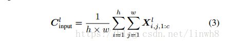

补充: 第一层squeeze操作,是将3d tensor 转化为 channel tensor。然后经过两层卷积提取特征。
red框的输出与HA的输入作multiply op后传入下一层。red框体现了HA-CNN的第三个特点: Joint learning of soft and hard attention
最后来看黑色框。作者 model the hard region attention as a transform matrix, 即公式(5), which allows for image cropping, translation and isotropic scaling operations by varying two scale factors (sh,sw) ( s h , s w ) and 2-D spatial position (tx,ty) ( t x , t y )

作者通过使用固定的 sh s h 与 sw s w 来限制模型复杂度,所以hard attention model 只需要考虑两个参数。目前输入是一个c-D vector
, 并且我们提取T个regions,所以蓝色部分的全连接层的参数便是2T*c 个参数。然后经过Tanh,最后获得2T输出 θ θ 。
补充: 作者将hard attention 给 model 成 一个变换矩阵,该矩阵主要有4个参数: sh s h 、 sw s w 、 tx t x 、 ty t y 。 其中, sh s h 、 sw s w 用于固定region的大小,以限制模型的复杂度,所以hard attention learning 学的便是这两个t变量。所以,全连接层的输出是2T,再经过Tanh,将position转化为百分比,以方便定位region的位置,即输出的 θ θ 是T个region的位置信息
θ θ 按照虚线传输回之前的结点,然后分成T个parts根据红线输入到各个Local branches做add op。
更正:现在解释一下HA-CNN的虚线与红线。虚线部分,引用原文如下:
The hard region attention is enforced on that of the corresponding network block to generate T different parts which are subsequently fed into the corresponding streams of the local branch.
这个“enforce” and then “generate T parts” 很迷,应该是没讲清楚。作者的意思应该是从HA模块传回的 θ θ 是regions的position info,然后从所到达的network block的当前feature map中获得region,将他们分别resize 成24x28x32、12x14x d1 d 1 、6x7x d2 d 2 ,传入local分支中与local feature做 add op。这一过程可以用公式(6) 描述
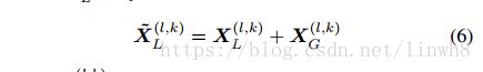
补充: 为什么做这个加法?作者的意思将global branch 学习到的东西分享给local branch,相当于分享了global branch 的学习能力,所以这样可以减少local branch的层数,继而减少参数量。
模型的参数训练,如公式(7)
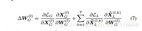
公式(6) 与 公式 (7) 体现了HA-CNN的第四个特点:Cross-attention interaction learning scheme between attention selection and feature representation
HA-CNN on ReID
- A test probe image Ip I p , A set of test gallery image {Igi} { I i g }
(1) We first compute their corresponding 1,024-D feature vectors by forward-feeding the images to a trained HA-CNN model, denoted as xp=[xpg;xpl] x p = [ x g p ; x l p ] and {xgi=[xgg;xgl]} { x i g = [ x g g ; x l g ] }
(2) We then compute L2 normalisation on the global and local features, respectively.
(3) Lastly, we compute the crosscamera matching distances between xp x p and xgi x i g by the L2distance.
(4) We then rank all gallery images in ascendant order by their L2 distances to the probe image.
Experiment
实现细节:
1. All person images are resized to 160×64;
2. we set the width of Inception units at the 1st/2nd/3rd levels as: d1 =128, d2 = 256 and d3 = 384;
3. we use T = 4 regions for hard attention;
4. In each stream, we fix the size of three levels of hard attention
as 24×28, 12×14 and 6×7;
5. For model optimisation, we use the ADAM algorithm at the initial learning rate 5×10⁻⁴ with the two moment terms β1 = 0:9 and β2 = 0:999;
6. We set the batch size to 32, epoch to 150, momentum to 0.9;
7. , we do not adopt any data argumentation methods (e.g. scaling, rotation, flipping, and colour distortion), neither model pre-training.
实验结果:
Market-1501

DukeMTMC-ReID

CUHK03
这个比较特殊,原本是1367/100 training/test split,作者采用的是767/700

Attention Evaluation

CAIL Evaluation

Joint of global and local feature Evaluation

模型参数对比

Visulisation
Soft attention捕捉具有强烈区分性的特征,如那一坨彩色的东西;
Hard attention能够定位身体部位,如那四个框框
