吴恩达cs229|编程作业第三周（Python）

练习三：多分类和神经网络

目录

1.包含的文件

2.多分类问题

3.神经网络

1.包含的文件

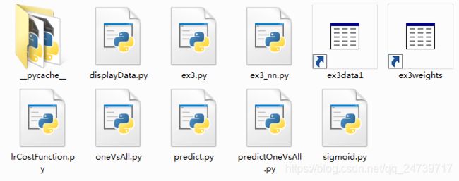
文件名	含义
ex3.py	逻辑回归多分类
ex3_nn.py	神经网络分类
ex3data1.mat	手写数字集
ex3weights.mat	神经网络初始权重
displayData.py	可视化数据
sigmoid.py	Sigmoid函数
lrCostFunction.py	多分类逻辑回归代价函数
oneVsAll.py	训练多分类器
predictOneVsAll.py	使用多分类器进行预测
predict.py	使用神经网络预测

红色部分需要自己填写。

2.多分类问题

• 需要的包以及初始化：

import matplotlib.pyplot as plt
import numpy as np
import scipy.io as scio

import displayData as dd
import lrCostFunction as lCF
import oneVsAll as ova
import predictOneVsAll as pova

plt.ion()

# Setup the parameters you will use for this part of the exercise
input_layer_size = 400  # 20x20 input images of Digits
num_labels = 10         # 10 labels, from 0 to 9
                        # Note that we have mapped "0" to label 10

2.1加载数据并可视化

• 可视化程序displayData.py：

import matplotlib.pyplot as plt
import numpy as np


def display_data(x):
    (m, n) = x.shape

    # Set example_width automatically if not passed in
    example_width = np.round(np.sqrt(n)).astype(int)
    example_height = (n / example_width).astype(int)

    # Compute the number of items to display
    display_rows = np.floor(np.sqrt(m)).astype(int)
    display_cols = np.ceil(m / display_rows).astype(int)

    # Between images padding
    pad = 1

    # Setup blank display
    display_array = - np.ones((pad + display_rows * (example_height + pad),
                              pad + display_rows * (example_height + pad)))

    # Copy each example into a patch on the display array
    curr_ex = 0
    for j in range(display_rows):
        for i in range(display_cols):
            if curr_ex > m:
                break

            # Copy the patch
            # Get the max value of the patch
            max_val = np.max(np.abs(x[curr_ex]))
            display_array[pad + j * (example_height + pad) + np.arange(example_height),
                          pad + i * (example_width + pad) + np.arange(example_width)[:, np.newaxis]] = \
                          x[curr_ex].reshape((example_height, example_width)) / max_val
            curr_ex += 1

        if curr_ex > m:
            break

    # Display image
    plt.figure()
    plt.imshow(display_array, cmap='gray', extent=[-1, 1, -1, 1])
    plt.axis('off')

• 测试代码：

# ===================== Part 1: Loading and Visualizing Data =====================
# We start the exercise by first loading and visualizing the dataset.
# You will be working with a dataset that contains handwritten digits.
#
# Load Training Data
print('Loading and Visualizing Data ...')

data = scio.loadmat('ex3data1.mat')  #读取训练集 包括两部分 输入特征和标签
X = data['X']   #提取输入特征 5000*400的矩阵  5000个训练样本 每个样本特征维度为400 一行代表一个训练样本
y = data['y'].flatten() #提取标签 data['y']是一个5000*1的2维数组 利用flatten()将其转换为有5000个元素的一维数组
 
m = y.size  #训练样本的数量
 
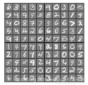
# 随机抽取100个训练样本 进行可视化
rand_indices = np.random.permutation(range(m)) #获取0-4999 5000个无序随机索引
selected = X[rand_indices[0:100], :]  #获取前100个随机索引对应的整条数据的输入特征
 
dd.display_data(selected)   #调用可视化函数 进行可视化

input('Program paused. Press ENTER to continue')

• 测试结果：

2.2向量化逻辑回归

• 回想一下，在(非正则化)逻辑回归中，代价函数是

• 其中：

                     

• 我们可以用矩阵乘法快速地计算出所有的例子，我们定义：

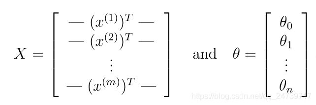
• 然后,通过计算矩阵乘积Xθ，得到：

• 回想一下(非正则化)逻辑回归代价的梯度是一个向量，其中第j个元素定义为：

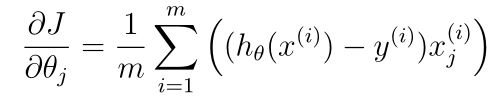
• 向量化梯度为：

• 其中：

• 为理解推导过程的最后一步,让β=θ(h (x (i))−y (i))，这样变形为：

• 其中：

• 为了向量化正则化逻辑回归，先回忆一下，对于正则化逻辑回归，代价函数定义为：

• 相应地,正规化的逻辑回归的偏导数为θj被定义为：

如何向量化，参照未带正则化的逻辑回归。

• 在lrCostFunction.py中编写代码计算代价函数和梯度：

import numpy as np
from sigmoid import *

def lr_cost_function(theta, X, y, lmd):
    m = y.size

    # You need to return the following values correctly
    cost = 0
    grad = np.zeros(theta.shape)

    # ===================== Your Code Here =====================
    # Instructions : Compute the cost of a particular choice of theta
    #                You should set cost and grad correctly.
    #
    h_out= np.dot(X,theta)#使用点乘 生成一维的数组  
    theta_lmd = theta[1:]#第一个theta不正则化
    #在前面的基础上加上正则项
    cost = -np.mean((y*np.log(sigmoid(h_out))+(1-y)*np.log(1-sigmoid(h_out))),axis=0)+lmd/(2*m)*(theta_lmd*theta_lmd).sum()
 
    error = sigmoid(h_out)- y# sigmoid(a0+a1x1+...) 再与y求偏差
    error_2d =  error.reshape(m,1)#转换成2维数组进行乘法
    error_all = error_2d*X#是一个 m*n大小的数组
    #j>=1加上正则化项 j=0不加
    grad[0] = (1/m)*error_all[:,0].sum(axis=0)
    grad[1:] = (1/m)*error_all[:,1:].sum(axis=0)+lmd/m*theta_lmd

    # =========================================================

    return cost, grad

• sigmoid.py为：

import numpy as np

def sigmoid(z):
    return 1 / (1 + np.exp(-z))

• 测试代码为：

# ===================== Part 2-a: Vectorize Logistic Regression =====================
# In this part of the exercise, you will reuse your logistic regression
# code from the last exercise. Your task here is to make sure that your
# regularized logistic regression implementation is vectorized. After
# that, you will implement one-vs-all classification for the handwritten
# digit dataset
#

# Test case for lrCostFunction
print('Testing lrCostFunction()')

theta_t = np.array([-2, -1, 1, 2])
X_t = np.c_[np.ones(5), np.arange(1, 16).reshape((3, 5)).T/10]
y_t = np.array([1, 0, 1, 0, 1])
lmda_t = 3
cost, grad = lCF.lr_cost_function(theta_t, X_t, y_t, lmda_t)

np.set_printoptions(formatter={'float': '{: 0.6f}'.format})
print('Cost: {:0.7f}'.format(cost))
print('Expected cost: 2.534819')
print('Gradients:\n{}'.format(grad))
print('Expected gradients:\n[ 0.146561 -0.548558 0.724722 1.398003]')

input('Program paused. Press ENTER to continue')

• 测试结果：

Testing lrCostFunction()
Cost: 2.5348194
Expected cost: 2.534819
Gradients:
[ 0.146561 -0.548558  0.724722  1.398003]
Expected gradients:
[ 0.146561 -0.548558 0.724722 1.398003]

2.3One vs All 分类训练

• 编写逻辑回归多分类器的训练程序oneVsAll.py

import scipy.optimize as opt
import lrCostFunction as lCF
from sigmoid import *

def one_vs_all(X, y, num_labels, lmd):
    # Some useful variables
    (m, n) = X.shape

    # You need to return the following variables correctly
    all_theta = np.zeros((num_labels, n + 1))

    # Add ones to the X data 2D-array
    X = np.c_[np.ones(m), X]

    for i in range(num_labels):
        print('Optimizing for handwritten number {}...'.format(i))
        # ===================== Your Code Here =====================
        # Instructions : You should complete the following code to train num_labels
        #                logistic regression classifiers with regularization
        #                parameter lambda
        #
        #
        # Hint: you can use y == c to obtain a vector of True(1)'s and False(0)'s that tell you
        #       whether the ground truth is true/false for this class
        #
        # Note: For this assignment, we recommend using opt.fmin_cg to optimize the cost
        #       function. It is okay to use a for-loop (for c in range(num_labels) to
        #       loop over the different classes
        #
         # Optimize
        def cost_func(theta_t):
            return lCF.lr_cost_function(theta_t, X, y_t, lmda_t)[0]
        
        def grad_func(theta_t):
            return lCF.lr_cost_function(theta_t, X, y_t, lmda_t)[1]       
        
        theta_t = all_theta[i,:]
        if i==0:
            iclass = 10
        else:
            iclass = i
        y_t = np.array([1 if x == iclass else 0 for x in y])
        lmda_t = lmd       
        theta, *unused = opt.fmin_cg(f=cost_func, fprime=grad_func, x0=theta_t, maxiter=100, full_output=True, disp=False) 
        all_theta[i,:] = theta
        # ============================================================    
        print('Done')

    return all_theta

• 测试代码：

# ===================== Part 2-b: One-vs-All Training =====================
print('Training One-vs-All Logistic Regression ...')

lmd = 0.1
all_theta = ova.one_vs_all(X, y, num_labels, lmd)#返回训练好的参数

input('Program paused. Press ENTER to continue')

• 运行结果

Training One-vs-All Logistic Regression ...
Optimizing for handwritten number 0...
Done
Optimizing for handwritten number 1...
Done
Optimizing for handwritten number 2...
Done
Optimizing for handwritten number 3...
Done
Optimizing for handwritten number 4...
Done
Optimizing for handwritten number 5...
Done
Optimizing for handwritten number 6...
Done
Optimizing for handwritten number 7...
Done
Optimizing for handwritten number 8...
Done
Optimizing for handwritten number 9...
Done

2.4One vs All 分类预测

• 编写测试程序predictOneVsAll.py

import numpy as np


def predict_one_vs_all(all_theta, X):
    m = X.shape[0]
    num_labels = all_theta.shape[0]

    # You need to return the following variable correctly;
    p = np.zeros(m)

    # Add ones to the X data matrix
    X = np.c_[np.ones(m), X]

    # ===================== Your Code Here =====================
    # Instructions : Complete the following code to make predictions using
    #                your learned logistic regression parameters (one vs all).
    #                You should set p to a vector of predictions (from 1 to
    #                num_labels)
    #
    # Hint : This code can be done all vectorized using the max function
    #        In particular, the max function can also return the index of the
    #        max element, for more information see 'np.argmax' function.
    #
    num = np.dot(X,all_theta.T) #求出矩阵
    p = np.argmax(num,axis=1)#求出行的最大值索引
    p[p==0] = num_labels #第0类 用最大类别表示

    return p

• 测试程序：

# ===================== Part 3: Predict for One-Vs-All =====================

pred = pova.predict_one_vs_all(all_theta, X)

print('Training set accuracy: {}'.format(np.mean(pred == y)*100))

input('ex3 Finished. Press ENTER to exit')

• 测试结果：

Training set accuracy: 96.06

3.神经网络

• 导入需要的包以及初始化：

import matplotlib.pyplot as plt
import numpy as np
import scipy.io as scio

import displayData as dd
import predict as pd

plt.ion()

# Setup the parameters you will use for this part of the exercise
input_layer_size = 400  # 20x20 input images of Digits
hidden_layer_size = 25  # 25 hidden layers
num_labels = 10         # 10 labels, from 0 to 9
                        # Note that we have mapped "0" to label 10

• 查看可视化程序displayData.py

def display_data(x):
    (m, n) = x.shape   #100*400
 
    example_width = np.round(np.sqrt(n)).astype(int) #每个样本显示宽度 round()四舍五入到个位 并转换为int
    example_height = (n / example_width).astype(int) #每个样本显示高度  并转换为int
 
    #设置显示格式 100个样本 分10行 10列显示
    display_rows = np.floor(np.sqrt(m)).astype(int)
    display_cols = np.ceil(m / display_rows).astype(int)
 
    # 待显示的每张图片之间的间隔
    pad = 1
 
    # 显示的布局矩阵 初始化值为-1
    display_array = - np.ones((pad + display_rows * (example_height + pad),
                              pad + display_rows * (example_height + pad)))
 
    # Copy each example into a patch on the display array
    curr_ex = 0
    for j in range(display_rows):
        for i in range(display_cols):
            if curr_ex > m:
                break
 
            # Copy the patch
            # Get the max value of the patch
            max_val = np.max(np.abs(x[curr_ex]))
            display_array[pad + j * (example_height + pad) + np.arange(example_height),
                          pad + i * (example_width + pad) + np.arange(example_width)[:, np.newaxis]] = \
                          x[curr_ex].reshape((example_height, example_width)) / max_val
            curr_ex += 1
 
        if curr_ex > m:
            break
 
    # 显示图片
    plt.figure()
    plt.imshow(display_array, cmap='gray', extent=[-1, 1, -1, 1])
    plt.axis('off')

• 数据可视化测试：

# ===================== Part 1: Loading and Visualizing Data =====================
# We start the exercise by first loading and visualizing the dataset.
# You will be working with a dataset that contains handwritten digits.
#

# Load Training Data
print('Loading and Visualizing Data ...')

data = scio.loadmat('ex3data1.mat')
X = data['X']
y = data['y'].flatten()
m = y.size

# Randomly select 100 data points to display
rand_indices = np.random.permutation(range(m))
selected = X[rand_indices[0:100], :]

dd.display_data(selected)

input('Program paused. Press ENTER to continue')

• 测试结果：

• 加载神经网络参数：

# ===================== Part 2: Loading Parameters =====================
# In this part of the exercise, we load some pre-initiated
# neural network parameters

print('Loading Saved Neural Network Parameters ...')

data = scio.loadmat('ex3weights.mat')
theta1 = data['Theta1']
theta2 = data['Theta2']

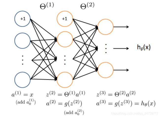
• 编写神经网络的前向传播程序 predict.py

import numpy as np
from sigmoid import *

def predict(theta1, theta2, x):
    # Useful values
    m = x.shape[0]
    num_labels = theta2.shape[0]

    # You need to return the following variable correctly
    p = np.zeros(m)

    # ===================== Your Code Here =====================
    # Instructions : Complete the following code to make predictions using
    #                your learned neural network. You should set p to a
    #                1-D array containing labels between 1 to num_labels.
    #
    # Add ones to the X data matrix
    X = np.c_[np.ones(m), x]
    
    layer_1 = np.dot(X,theta1.T)# (100*401)*(401*25) = 100*25
    
    hidden = np.c_[np.ones(m), layer_1] #增加1 变成隐藏层 100*26
    
    output = np.dot(hidden,theta2.T)# (100*26)*(26*10) = (100*10)
    
    p = np.argmax(output,axis=1)#求出行的最大值索引
    p[p==0] = num_labels #第0类 用最大类别表示

    return p

• 实现预测过程：

# ===================== Part 3: Implement Predict =====================
# After training the neural network, we would like to use it to predict
# the labels. You will now implement the "predict" function to use the
# neural network to predict the labels of the training set. This lets
# you compute the training set accuracy.

pred = pd.predict(theta1, theta2, X)

print('Training set accuracy: {}'.format(np.mean(pred == y)*100))

input('Program paused. Press ENTER to continue')

# To give you an idea of the network's output, you can also run
# thru the examples one at a time to see what it is predicting


def getch():
    import termios
    import sys, tty

    def _getch():
        fd = sys.stdin.fileno()
        old_settings = termios.tcgetattr(fd)
        try:
            tty.setraw(fd)
            ch = sys.stdin.read(1)
        finally:
            termios.tcsetattr(fd, termios.TCSADRAIN, old_settings)
        return ch

    return _getch()

# Randomly permute examples
rp = np.random.permutation(range(m))
for i in range(m):
    print('Displaying Example image')
    example = X[rp[i]]
    example = example.reshape((1, example.size))
    dd.display_data(example)

    pred = pd.predict(theta1, theta2, example)
    print('Neural network prediction: {} (digit {})'.format(pred, np.mod(pred, 10)))

    s = input('Paused - press ENTER to continue, q + ENTER to exit: ')
    if s == 'q':
        break

• 测试结果：

Training set accuracy: 96.06

 

注：所有代码及说明PDF在全部更新完后统一上传。