python计算机视觉编程（三）——Harris角点 SIFT 匹配地理标记图像

准备

使用的到一些函数在文末给出

VLFeat

使用开源工具包VLFeat提供的二进制文件来计算图像的SIFT特征
链接: http://www.vlfeat.org/建议下载20以前的版本，最新版本产生的SIFT特征文本为空
将bin目录下对应的系统文件夹复制出来

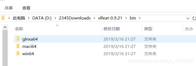
之后将process_image函数中路径改成相应的位置

pydot工具包

用pydot可以直接可视化他们直接的关联
1.安装graphviz

pip install graphviz

2.安装graphviz软件，地址在：https://graphviz.gitlab.io/_pages/Download/Download_windows.html

3.把安装后的graphviz软件的bin目录设为环境变量，重启。

4.安装pydot

pip install pydot

由于sift速度较慢，建议把图片压缩后使用！！！

Harris角点

原理

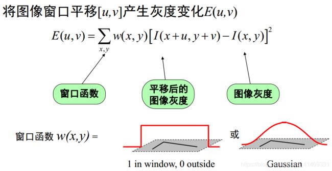
角点检测最原始的想法就是取某个像素的一个邻域窗口，当这个窗口在各个方向上进行小范围移动时，观察窗口内平均的像素灰度值的变化（即，E(u,v)）。

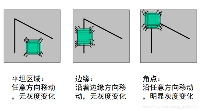
从上图可知，我们可以将一幅图像大致分为三个区域（‘flat’，‘edge’，‘corner’），这三个区域变化是不一样的。

将函数二维泰勒展开

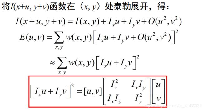
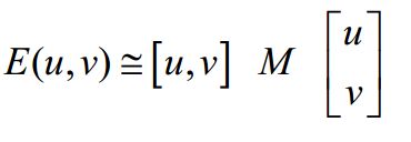
于是对于局部微小的移动量 [u,v]， 可以近似得到下面的表达：

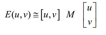
其中M是 22 矩阵， 可由图像的导数求得：

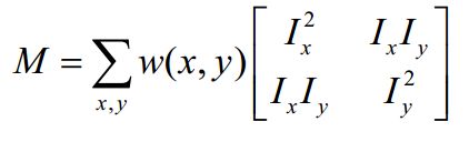
窗口移动导致的图像变化量： 实对称矩阵M的特征值分析

记M的特征值为 λ 1, λ 2

定义： 角点响应函数R


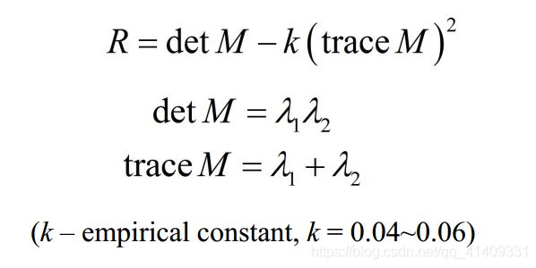
角点计算流程:
对角点响应函数R进行阈值处理：
R > threshold
提取R的局部极大值

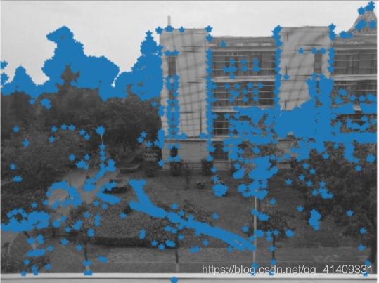
代码实现

Harris角点检测

from pylab import *
from PIL import Image
from scipy.ndimage import filters
from sift import *

# 读入图像
im = array(Image.open('123.jpg').convert('L'))

# 检测harris角点
harrisim = compute_harris_response(im)
filtered_coords = get_harris_points(harrisim,6)

plot_harris_points(im, filtered_coords)

Harris角点匹配

from pylab import *
from PIL import Image
from pylab import *
from numpy import *
from scipy.ndimage import filters
from sift import *


im1 = array(Image.open("123.jpg").convert("L"))
im2 = array(Image.open("456.jpg").convert("L"))

# resize加快匹配速度
im1 = imresize(im1, (int(im1.shape[1]/2), int(im1.shape[0]/2)))
im2 = imresize(im2, (int(im2.shape[1]/2), int(im2.shape[0]/2)))

wid = 5
harrisim = compute_harris_response(im1, 5)
filtered_coords1 = get_harris_points(harrisim, wid+1)
d1 = get_descriptors(im1, filtered_coords1, wid)

harrisim = compute_harris_response(im2, 5)
filtered_coords2 = get_harris_points(harrisim, wid+1)
d2 = get_descriptors(im2, filtered_coords2, wid)

print ('starting matching')
matches = match_twosided(d1, d2)

figure()
gray() 
plot_matches(im1, im2, filtered_coords1, filtered_coords2, matches)
show()

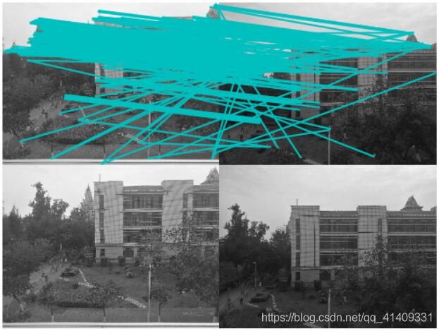
可以看出特征点的匹配比较混乱，下文将介绍SIFT，它的效果非常不错，缺点就是比较耗时。

SIFT

原理

SIFT算法实现特征匹配主要有三个流程， 1、 提取关键点； 2、 对关键点附加
详细的信息（ 局部特征） ， 即描述符； 3、 通过特征点（ 附带上特征向量的关
键点） 的两两比较找出相互匹配的若干对特征点， 建立景物间的对应关系。
1.高斯模糊
高斯模糊是在Adobe Photoshop等图像处理软件中广泛使用的处理
效果， 通常用它来减小图像噪声以及降低细节层次。 这种模糊技术生成
的图像的视觉效果是好像经过一个半透明的屏幕观察图像。
二维高斯函数
高斯卷积核是实现尺度变换的唯一变换核，并且是唯一的线性核。高斯模糊是一种图像滤波器，它使用正态分布(高斯函数)计算模糊模板，并使用该模板与原图像做卷积运算，达到模糊图像的目的。

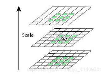
2.尺度空间
尺度空间理论最早于1962年提出， 其主要思想是通过对原始图像进行尺度变换， 获得图像多尺度下的空间表示。从而实现边缘、 角点检测和不同分辨率上的特征提取， 以满足特征点的尺度不变性。尺度空间中各尺度图像的模糊程度逐渐变大， 能够模拟人在距离目标由近到远时目标在视网膜上的形成过程。尺度越大图像越模糊。
2.1高斯金字塔
高斯金子塔的构建过程可分为两步：
（ 1） 对图像做高斯平滑；
（ 2） 对图像做降采样。
为了让尺度体现其连续性， 在简单下采样的基础上加上了高斯滤波。一幅图像可以产生几组（ octave）图像， 一组图像包括几层（ interval） 图像。

高斯图像金字塔共o组、 s层，则有：

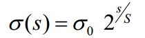
σ——尺度空间坐标；
s——sub-level层坐标；
σ0——初始尺度；
S——每组层数（ 一般为3~5）
最后可将组内和组间尺度归为：

i——金字塔组数
n——每一组的层数
2.2DOG
使用高斯金字塔每组中相邻上下两层图像相减，得到高斯差分图像，进行极值检测。


可以通过高斯差分图像看出图像上的像素值变化情况。 （ 如果没有变化， 也就没有特征。 特征必须是变化尽可能多的点。 ）DOG图像描绘的是目标的轮廓。
2.3DoG的局部极值点
特征点是由DOG空间的局部极值点组成的。 为了寻找DoG函数的极值点，每一个像素点要和它所有的相邻点比较， 看其是否比它的图像域和尺度域的相邻点大或者小。中间的检测点和它同尺度的8个相邻点和上下相邻尺度对应的9× 2个点共26个点比较， 以确保在尺度空间和二维图像空间都检测到极值点。

3关键点定位
3.1去除边缘响应
由于DoG函数在图像边缘有较强的边缘响应， 因此需要排除边缘响应。DoG函数的峰值点在边缘方向有较大的主曲率， 而在垂直边缘的方向有较小的主曲率。主曲率可以通过计算在该点位置尺度的2×2的Hessian矩阵得到， 导数由采样点相邻差来估计：

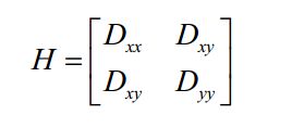
Dxx 表示DOG金字塔中某一尺度的图像x方向求导两次
D的主曲率和H的特征值成正比。 令 α ， β为特征值， 则

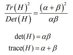
该值在两特征值相等时达最小。 Lowe论文中建议阈值T为1.2， 即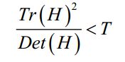时保留关键点， 反之剔除
4方向分配
通过尺度不变性求极值点， 可以使其具有缩放不变的性质。 而利
用关键点邻域像素的梯度方向分布特性， 可以为每个关键点指定方向参数
方向， 从而使描述子对图像旋转具有不变性。
像素点的梯度表示：

梯度幅值：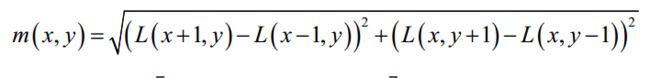
梯度方向：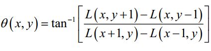
通过求每个极值点的梯度来为极值点赋予方向。
方向直方图的生成
确定关键点的方向采用梯度直方图统计法， 统计以关键点为原点， 一定区域内的图像像素点对关键点方向生成所作的贡献。
关键点主方向： 极值点周围区域梯度直方图的主峰值也是特征点方向。
关键点辅方向： 在梯度方向直方图中， 当存在另一个相当于主峰值80%能量的峰值时， 则将这个方向认为是该关键点的辅方向。
这可以增强匹配的鲁棒性， Lowe的论文指出大概有15%关键点具有
多方向， 但这些点对匹配的稳定性至为关键。
5关键点特征描述
下图是一个SIFT描述子事例。 其中描述子由2× 2× 8维向量表征， 也即是2× 2个8方向的方向直方图组成。 左图的种子点由8× 8单元组成。 每一个小格都代表了特征点邻域所在的尺度空间的一个像素， 箭头方向代表了像素梯度方向， 箭头长度代表该像素的幅值。 然后在4×4的窗口内计算8个方向的梯度方向直方图。 绘制每个梯度方向的累加可形成一个种子点， 如右图所示： 一个特征点由4个种子点的信息所组成。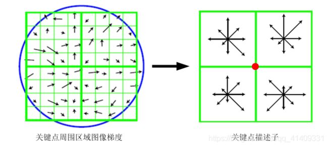
6关键点匹配
分别对模板图（ 参考图， reference image） 和实时图（ 观测图，observation image） 建立关键点描述子集合。 目标的识别是通过两点集内关键点描述子的比对来完成。 具有128维的关键点描述子的相似性度量采用欧式距离。

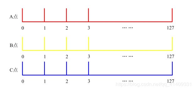
穷举匹配

模板图中关键点描述子：

实时图中关键点描述子：

任意两描述子相似性度量：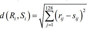
要得到配对的关键点描述子需满足：
关键点的匹配可以采用穷举法来完成， 但是这样耗费的时间太多， 一
般都采用kd树的数据结构来完成搜索。 搜索的内容是以目标图像的关
键点为基准， 搜索与目标图像的特征点最邻近的原图像特征点和次邻
近的原图像特征点。
Kd树是一个平衡二叉树

代码实现

SIFT特征检测

from PIL import Image
from pylab import *
from numpy import *
import os
from sift import *

imname = '123.jpg'
im1 = array(Image.open(imname).convert('L'))
process_image(imname, 'empire.sift')
l1,d1 = read_features_from_file('empire.sift')

figure()
gray()
plot_features(im1, l1, circle=True)
show()

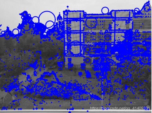
SIFT特征匹配

from PIL import Image
from pylab import *
import sys
import sift

if len(sys.argv) >= 3:
  im1f, im2f = sys.argv[1], sys.argv[2]
else:
  im1f = '123.jpg'
  im2f = '456.jpg'
im1 = array(Image.open(im1f))
im2 = array(Image.open(im2f))

sift.process_image(im1f, 'out_sift_1.txt')
l1, d1 = sift.read_features_from_file('out_sift_1.txt')
figure()
gray()
subplot(121)
sift.plot_features(im1, l1, circle=False)

sift.process_image(im2f, 'out_sift_2.txt')
l2, d2 = sift.read_features_from_file('out_sift_2.txt')
subplot(122)
sift.plot_features(im2, l2, circle=False)

matches = sift.match_twosided(d1, d2)
print ('{} matches'.format(len(matches.nonzero()[0])))

figure()
gray()
sift.plot_matches(im1, im2, l1, l2, matches, show_below=True)
show()

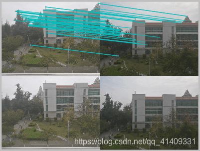
明显与Harris相比特征点的匹配更为准确

Harris与SIFT的对比

from PIL import Image
from pylab import *
import sift

imname = '123.jpg'
im = array(Image.open(imname).convert('L'))
sift.process_image(imname, 'empire.sift')
l1, d1 = sift.read_features_from_file('empire.sift')

figure()
gray()
subplot(131)
sift.plot_features(im, l1, circle=False)
subplot(132)
sift.plot_features(im, l1, circle=True)

# 检测harris角点
harrisim = sift.compute_harris_response(im)

subplot(133)
filtered_coords = sift.get_harris_points(harrisim, 6, 0.1)
imshow(im)
plot([p[1] for p in filtered_coords], [p[0] for p in filtered_coords], '*')
axis('off')

show()

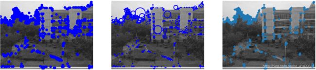
三图分别为SIFT特征，用圆圈表示SIFT特征，Harris角点
明显的看出SIFT特征数量较多，同时通过上文的匹配点匹配效果来看，SIFT的效果远远优于Harris，缺点是运行时间长

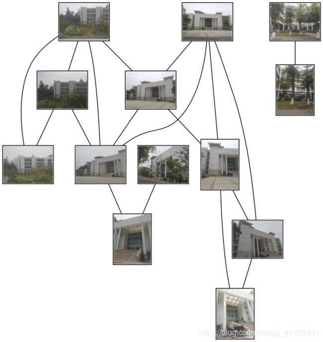
匹配地理标记图像

可以通过匹配多张图片的描述子，找到他们之间的对应关系

from pylab import *
from PIL import Image
import sift
import pydot
import os

def get_imlist(path):
        
    return [os.path.join(path,f) for f in os.listdir(path) if f.endswith('.jpg')]

download_path = "D:/opencv-py/image"  
path = "D:/opencv-py/image"  

imlist = get_imlist(download_path)
nbr_images = len(imlist)

featlist = [imname[:-3] + 'sift' for imname in imlist]
for i, imname in enumerate(imlist):
    sift.process_image(imname, featlist[i])

matchscores = zeros((nbr_images, nbr_images))

for i in range(nbr_images):
    for j in range(i, nbr_images):  # only compute upper triangle
        print ('comparing ', imlist[i], imlist[j])
        l1, d1 = sift.read_features_from_file(featlist[i])
        l2, d2 = sift.read_features_from_file(featlist[j])
        matches = sift.match_twosided(d1, d2)
        nbr_matches = sum(matches > 0)
        print ('number of matches = ', nbr_matches)
        matchscores[i, j] = nbr_matches
print ("The match scores is: \n", matchscores)

for i in range(nbr_images):
    for j in range(i + 1, nbr_images):  # no need to copy diagonal
        matchscores[j, i] = matchscores[i, j]
threshold = 2  # min number of matches needed to create link

g = pydot.Dot(graph_type='graph')  # don't want the default directed graph

for i in range(nbr_images):
    for j in range(i + 1, nbr_images):
        if matchscores[i, j] > threshold:
            # first image in pair
            im = Image.open(imlist[i])
            im.thumbnail((100, 100))
            filename = path + str(i) + '.png'
            im.save(filename)  # need temporary files of the right size
            g.add_node(pydot.Node(str(i), fontcolor='transparent', shape='rectangle', image=filename))

            im = Image.open(imlist[j])
            im.thumbnail((100, 100))
            filename = path + str(j) + '.png'
            im.save(filename)  # need temporary files of the right size
            g.add_node(pydot.Node(str(j), fontcolor='transparent', shape='rectangle', image=filename))

            g.add_edge(pydot.Edge(str(i), str(j)))
g.write_png('whitehouse.png')

一些用到的函数

sift.py

from PIL import Image
import os
from numpy import *
from pylab import *
from scipy.ndimage import filters
def imresize(im,sz):
    pil_im = Image.fromarray(uint8(im))
    
    return array(pil_im.resize(sz))

def compute_harris_response(im,sigma=3):
    imx = zeros(im.shape)
    filters.gaussian_filter(im, (sigma,sigma), (0,1), imx)
    imy = zeros(im.shape)
    filters.gaussian_filter(im, (sigma,sigma), (1,0), imy)
    
    Wxx = filters.gaussian_filter(imx*imx,sigma)
    Wxy = filters.gaussian_filter(imx*imy,sigma)
    Wyy = filters.gaussian_filter(imy*imy,sigma)
    
    Wdet = Wxx*Wyy - Wxy**2
    Wtr = Wxx + Wyy
    
    return Wdet / Wtr

def get_harris_points(harrisim,min_dist=10,threshold=0.1):
    corner_threshold = harrisim.max() * threshold
    harrisim_t = (harrisim > corner_threshold) * 1
    
    coords = array(harrisim_t.nonzero()).T
    
    candidate_values = [harrisim[c[0],c[1]] for c in coords]
    
    index = argsort(candidate_values)[::-1]
    
    allowed_locations = zeros(harrisim.shape)
    allowed_locations[min_dist:-min_dist,min_dist:-min_dist] = 1
    
    filtered_coords = []
    for i in index:
        if allowed_locations[coords[i,0],coords[i,1]] == 1:
            filtered_coords.append(coords[i])
            allowed_locations[(coords[i,0]-min_dist):(coords[i,0]+min_dist), 
                        (coords[i,1]-min_dist):(coords[i,1]+min_dist)] = 0
    
    return filtered_coords


def plot_harris_points(image,filtered_coords):
    """ Plots corners found in image. """
    
    figure()
    gray()
    imshow(image)
    plot([p[1] for p in filtered_coords],[p[0] for p in filtered_coords],'*')
    axis('off')
    show()
def get_descriptors(image,filtered_coords,wid=5):
    """ For each point return pixel values around the point
        using a neighbourhood of width 2*wid+1. (Assume points are 
        extracted with min_distance > wid). """
    
    desc = []
    for coords in filtered_coords:
        patch = image[coords[0]-wid:coords[0]+wid+1,
                            coords[1]-wid:coords[1]+wid+1].flatten()
        desc.append(patch)
    
    return desc
def match(desc1,desc2,threshold=0.5):
    """ For each corner point descriptor in the first image, 
        select its match to second image using
        normalized cross correlation. """
    
    n = len(desc1[0])
    
    # pair-wise distances
    d = -ones((len(desc1),len(desc2)))
    for i in range(len(desc1)):
        for j in range(len(desc2)):
            d1 = (desc1[i] - mean(desc1[i])) / std(desc1[i])
            d2 = (desc2[j] - mean(desc2[j])) / std(desc2[j])
            ncc_value = sum(d1 * d2) / (n-1) 
            if ncc_value > threshold:
                d[i,j] = ncc_value
            
    ndx = argsort(-d)
    matchscores = ndx[:,0]
    
    return matchscores
def match_twosided(desc1,desc2,threshold=0.5):
    """ Two-sided symmetric version of match(). """
    
    matches_12 = match(desc1,desc2,threshold)
    matches_21 = match(desc2,desc1,threshold)
    
    ndx_12 = where(matches_12 >= 0)[0]
    
    # remove matches that are not symmetric
    for n in ndx_12:
        if matches_21[matches_12[n]] != n:
            matches_12[n] = -1
    
    return matches_12
def appendimages(im1,im2):
    """ Return a new image that appends the two images side-by-side. """
    
    # select the image with the fewest rows and fill in enough empty rows
    rows1 = im1.shape[0]    
    rows2 = im2.shape[0]
    
    if rows1 < rows2:
        im1 = concatenate((im1,zeros((rows2-rows1,im1.shape[1]))),axis=0)
    elif rows1 > rows2:
        im2 = concatenate((im2,zeros((rows1-rows2,im2.shape[1]))),axis=0)
    # if none of these cases they are equal, no filling needed.
    
    return concatenate((im1,im2), axis=1)
def plot_matches(im1,im2,locs1,locs2,matchscores,show_below=True):
    """ Show a figure with lines joining the accepted matches 
        input: im1,im2 (images as arrays), locs1,locs2 (feature locations), 
        matchscores (as output from 'match()'), 
        show_below (if images should be shown below matches). """
    
    im3 = appendimages(im1,im2)
    if show_below:
        im3 = vstack((im3,im3))
    
    imshow(im3)
    
    cols1 = im1.shape[1]
    for i,m in enumerate(matchscores):
        if m>0:
            plot([locs1[i][1],locs2[m][1]+cols1],[locs1[i][0],locs2[m][0]],'c')
    axis('off')
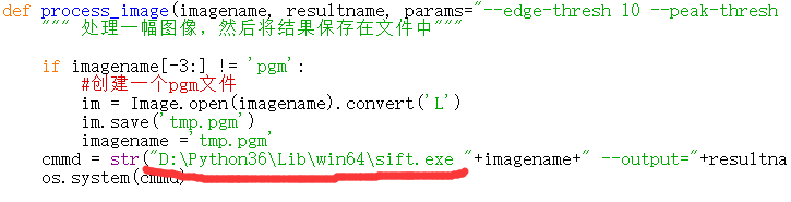
def process_image(imagename, resultname, params="--edge-thresh 10 --peak-thresh 5"):
    """ 处理一幅图像，然后将结果保存在文件中"""

    if imagename[-3:] != 'pgm':
        #创建一个pgm文件
        im = Image.open(imagename).convert('L')
        im.save('tmp.pgm')
        imagename ='tmp.pgm'
    cmmd = str("D:\Python36\Lib\win64\sift.exe "+imagename+" --output="+resultname+" "+params)
    os.system(cmmd)

def read_features_from_file(filename):
    """读取特征属性值，然后将其以矩阵的形式返回"""
    f = loadtxt(filename)
    return f[:,:4], f[:,4:] #特征位置，描述子

def write_featrues_to_file(filename, locs, desc):
    """将特征位置和描述子保存到文件中"""
    savetxt(filename, hstack((locs,desc)))

def plot_features(im, locs, circle=False):
    """显示带有特征的图像
       输入：im（数组图像），locs（每个特征的行、列、尺度和朝向）"""

    def draw_circle(c,r):
        t = arange(0,1.01,.01)*2*pi
        x = r*cos(t) + c[0]
        y = r*sin(t) + c[1]
        plot(x, y, 'b', linewidth=2)

    imshow(im)
    if circle:
        for p in locs:
            draw_circle(p[:2], p[2])
    else: 
        plot(locs[:,0], locs[:,1], 'ob')
    axis('off')