从程序中学习EKF-SLAM(一)
在一次课程的结课作业上,作业要求复写一个EKF-SLAM系统,我从中学到了好多知识。作为一个典型轻量级slam系统,这个小项目应该特别适合于slam系统入门,可以了解到经典卡尔曼滤波器在slam系统中的应用以及一个slam系统的重要组成部分。下面,我将以原理+代码形式来介绍这个project,如有问题,欢迎讨论;如有错误,欢迎指出。
参考博客:EKF-SLAM原理
它的原代码是用matlab写的,已经上传GitHub:ekf_slm_inMATLAB
它的演示视频也已经上传YouTube:ekf_slmVideo_inMATLAB
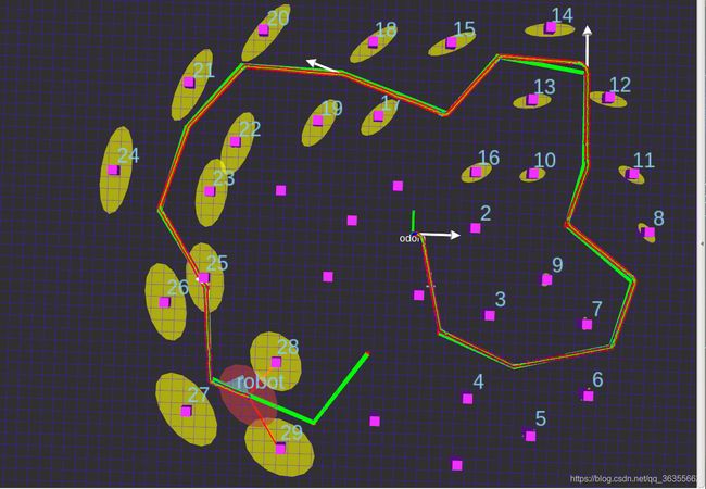
我的代码会放在GitHub上,请看最后一篇博客,下面的图片是显示效果。
一、整体框架
1.代码框架
首先从matlab的系统来说,它的核心分成了两个部分,这两个部分在C++工程中将会形成两个类。
在C++工程中,其中一个就是slam仿真器类,负责完成两个任务:
(1)计算car的真实位姿,收集观测的路标信息;
(2)对系统运行状态进行显示(在RVIZ中显示),协调。

另一个类就是核心了,扩展卡尔曼滤波器类,它负责两个非常重要的任务:
(1)估计位姿;
(2)更新位姿。

上面的两张图片里的内容是由各个子函数名构成的,这个类分别管理各自功能所属的子函数。
2.小车car的结构
下图是移动小车car在两个相邻时刻的位姿,其中 θ 1 {\theta}_1 θ1是两相邻时刻移动机器人绕圆弧运动的角度, θ 3 {\theta}_3 θ3是两相邻时刻移动机器航向角(朝向角head)的变化量。 l l l是左右轮之间的间距, d d d是右轮比左轮多走的距离。 r r r 是移动机器人圆弧运动的半径。

在本系统中,car的位姿是指 ( x , y , θ ) (x, y, \theta) (x,y,θ),它由两个控制量 ( V n , G n ) (V_n, G_n) (Vn,Gn)控制。其中,各个表示含义为:
(1) V n V_n Vn : car的前进线速度大小,在系统中是预先设定好的,此处是3m/s(这个在后面的配置文件里会说明);
(2) G n G_n Gn : car的转向角,用于控制car转向,它由据下一个新的路标点远近情况来决定。
那么,小车的位姿模型可以列成三个等式,如下所示:
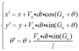
其中, d t dt dt是系统采样时间,此处是0.025秒。
二、程序主流程
1.准备
原matlab程序里有一个参数文件和一个数据文件,这里就统一用两个yaml文件来管理。首先,参数文件应该是最简单的,将原程序中的参数复制粘贴即可:
#%%% Configuration file
#%%% Permits various adjustments to parameters of the SLAM algorithm.
#%%% See ekfslam_sim.m for more information

#% control parameters
V: 3 #; % m/s
MAXG: rad(30*pi/180) #; % radians, maximum steering angle (-MAXG < g < MAXG)
RATEG: rad(20*pi/180) #; % rad/s, maximum rate of change in steer angle
WHEELBASE: 4 #; % metres, vehicle wheel-base
DT_CONTROLS: 0.025 #; % seconds, time interval between control signals控制信号之间的时间间隔

#% control noises
sigmaV: 0.3 #; % m/s
sigmaG: 0.03
#sigmaG: rad(3.0*pi/180) # ; % radians
#Q: [sigmaV^2 0; 0 sigmaG^2] #;

#% observation parameters
MAX_RANGE: 30.0 #; % metres
#DT_OBSERVE: 8*DT_CONTROLS #; % seconds, time interval between observations观测信号之间的间隔

#% observation noises
sigmaR: 0.1 #; % metres
sigmaB: rad(1.0*pi/180) #; % radians
#R: [sigmaR^2 0; 0 sigmaB^2] #;

#% data association innovation gates (Mahalanobis distances)
GATE_REJECT: 4.0 #; % maximum distance for association
GATE_AUGMENT: 25.0 #; % minimum distance for creation of new feature
#GATE_AUGMENT: 15.0
#% For 2-D observation:
#%   - common gates are: 1-sigma (1.0), 2-sigma (4.0), 3-sigma (9.0), 4-sigma (16.0)
#%   - percent probability mass is: 1-sigma bounds 40%, 2-sigma 86%, 3-sigma 99%, 4-sigma 99.9%.

#% waypoint proximity
AT_WAYPOINT: 1.0 #; % metres, distance from current waypoint at which to switch to next waypoint
NUMBER_LOOPS: 2 #; % number of loops through the waypoint list

#% switches
SWITCH_CONTROL_NOISE: 1 #; % if 0, velocity and gamma are perfect
SWITCH_SENSOR_NOISE: 1 #; % if 0, measurements are perfect
SWITCH_INFLATE_NOISE: 0 #; % if 1, the estimated Q and R are inflated (ie, add stabilising noise)
SWITCH_HEADING_KNOWN: 0 #; % if 1, the vehicle heading is observed directly at each iteration
SWITCH_ASSOCIATION_KNOWN: 0 #; % if 1, associations are given, if 0, they are estimated using gates
SWITCH_BATCH_UPDATE: 1 #; % if 1, process scan in batch, if 0, process sequentially
SWITCH_SEED_RANDOM: 0 #; % if not 0, seed the randn() with its value at beginning of simulation (for repeatability)
SWITCH_USE_IEKF: 0 #; % if 1, use iterated EKF for updates, if 0, use normal EKF
而这里的数据文件的读取有一点复杂,需要注意一下。它的yaml写法如下:
#保存路标点landmarks和路径点waypoints
#set of landmarks
lm: [[2.9922, -25.7009], [32.8988, -33.1776], [24.7991, -68.3801], [75.2664, -65.5763], [73.7087, -35.6698],
       [98.6308, 3.8941],  [49.4097, 26.9470], [80.2508, 59.9688], [54.7056, 88.6293], [13.2726, 80.8411],
       [-16.3224, 49.0654], [-65.8551, 83.6449], [-96.3847, 60.5919], [-76.1335, 36.2928], [-87.3505, -21.3396],
       [-103.5498, -32.2430], [-92.9579, -77.7259], [-55.8863, -55.9190], [-35.3255, -19.1589], [-56.1978, 16.3551],
       [-7.2882, 19.7819], [25.7336, 3.2710], [-19.5610, 80.1444], [-41.7506, 46.2325], [25.4021, 26.8543],
       [91.3870, 28.2385], [-13.7216, -79.0338], [-52.8454, -92.1833], [-86.1298, 15.0890], [-127.0053, 22.7018],
       [-25.9843, 4.7078], [56.3508, -17.4388], [51.6793, -83.1863], [21.31446, -96.3358], [48.1757, 57.9979]]

#set of waypoints
wp: [[12.6496, -41.588], [44.7368, -54.9844], [85.5467, -45.0156], [93.6464, -17.2897], [64.9860, 5.7632],
       [71.8396, 31.6199], [71.2165, 70.5607], [33.5218, 76.4798], [12.9611, 51.5576], [-32.5218, 67.4455],
       [-74.8894, 69.0031], [-97.3193, 41.9003], [-107.5997, 6.3863], [-86.4159, -25.7009], [-83.9237, -64.0187],
       [-39.3754, -81.4642], [-17.5685, -51.5576]]
程序里用一种特殊的数据类型进行转换,这里就只贴出landmark的坐标读取程序了。使用方法看懂了之后其实非常简单,照着学,学着用就行了。
//获取路标点以及行驶点
double dimension=1.0;
XmlRpc::XmlRpcValue landmarks_xmlrpc;
XmlRpc::XmlRpcValue waypoints_xmlrpc;
//获取参数的值
handle.getParam("/ekf_simulator/lm", landmarks_xmlrpc);
handle.getParam("/ekf_simulator/wp", waypoints_xmlrpc);

if (landmarks_xmlrpc.getType() == XmlRpc::XmlRpcValue::TypeArray)
{
	landmarks_size = landmarks_xmlrpc.size();
	std::cout<<"We obtained "<
其中,需要注意的就只有三条语句(步骤就是两步,一是取出每一个点,二是之后进行数据类型的强制转换即可):
XmlRpc::XmlRpcValue point = landmarks_xmlrpc[i];
landmarks(0, i)=double(point[0])/dimension;
landmarks(1, i)=double(point[1])/dimension;
2.主程序
这是用C++写的run函数,就是整个系统的主流程。
void slam_simulator::run()
{//main loop
	//% stored data for off-line
	ekf_cal->initialise_store();
	while((iwp !=-1)&&(ros::ok()))
	{
		//compute true data
		compute_steering();
		//perform loops: if final waypoint reached, go back to first
		if((iwp==-1)&&(number_loops>1))
		{
			iwp=0;
			number_loops=number_loops-1;
		}
		ekf_cal->vehicle_model(velocity, G, dt);
		ekf_cal->add_control_noise(velocity, G, switch_control_noise);	//默认添加噪声
		ekf_cal->predict(dt);
		//ekf_cal->ukf_predict(dt);

		//if heading known, observe heading
		//ekf_cal->observe_heading(switch_heading_know);			//默认此函数不用,转向未知

		//EKF update step
		dtsum= dtsum + dt;
		if(dtsum>=dt_observe)
		{
			dtsum=0;
			get_observations();
			ekf_cal->add_observation_noise(switch_sensor_noise);
			if(switch_association_know == 1)
				ekf_cal->data_associate_known(ftag_visible);			//已知数据关联,路标观测顺序已知
			else ekf_cal->data_associate(gate_reject, gate_augment);		//默认进程

			if(switch_use_Iekf == 1)
				ekf_cal->update_iekf(5);
			else ekf_cal->update(switch_batch_update);				//默认进程
			//ekf_cal->ukf_update(switch_batch_update);

		}

		//offline data store
		ekf_cal->store_data();
		viz_state();
		viz_dataAssociation();
		odometry_publisher();
		viz_robotpose();
		//r.sleep();
	}
}
后面我将会以程序的调用顺序,分别讲解每一个子函数,然后解释其中的原理,这样来学习ukf。