K-近邻算法（一）

    在网上对这个算法有很多详尽的描述，而且在B站上还有相关的视频讲解，如这篇博客：here。这里，在这篇博客中，仅仅从简单的总结和应用方面来记录下这个最简单的机器学习算法。

1. 原理

1.1 数据集

在使用k近邻法(k-nearest neighbor, k-NN)来进行类别的分类的时候，要求我们的训练数据集是有标签的数据，即：每组训练数据都要有标准答案，知道所属的正确类别。

1.2 算法思想

    对于训练数据集中的每条数据，我们可以将之看作一个集合空间中的一个点，而这个空间的维度也就是每条数据的特征数目；同理，对与待测试的数据集的每条数据，也可看作该空间中的一个点，我们要得到这个点的正确分类，我们不妨直接计算该点到所有的有标签的点距离即可。
    然后，取最接近的K个训练集合中的点，根据这些点的所属类别的比例，来决定最终预测的点的类别即可。
    在B站中，这个视频确实思路很清晰，here，有兴趣可以了解。

2. 实践

2.1 约会网站配对效果判定

    海伦女士一直使用在线约会网站寻找适合自己的约会对象。尽管约会网站会推荐不同的任选，但她并不是喜欢每一个人。经过一番总结，她发现自己交往过的人可以进行如下分类：

• 不喜欢的人
• 魅力一般的人
• 极具魅力的人

datingTestSet.txt数据下载。该数据集来源于这篇博客：here。
不妨看看这个数据集的格式：

知道了K近邻的思路，有了数据集，就不妨开始编写程序吧。

# 数据包的导入
import numpy as np
def data_processing(filename = "datingTestSet.txt"):
   # 读取文件内容到列表中
   datas = []
   with open(filename, mode="r", encoding='utf-8') as f:
       lines = f.readlines()
       for line in lines:
           _ = line.split("\t")
           _[3] = _[3][:-1]
           datas.append(_)
   datas = np.array(datas)
   # 需要转换下数据类型，到可计算数据类型
   feature_dataset = datas[:, :-1].astype(np.float) 
   # feature_dataset.shape   (1000, 3)
   
   # 数据归一化处理
   max_reduce_curr = np.tile(np.max(feature_dataset, axis=0), (feature_dataset.shape[0], 1)) - feature_dataset
   # max_reduce_curr.shape   (1000, 3)
   max_reduce_min = np.tile(np.max(feature_dataset, axis=0) - np.min(feature_dataset, axis=0), (feature_dataset.shape[0], 1))
   # max_reduce_min.shape   (1000, 3)
   new_feature_dataset = max_reduce_curr / max_reduce_min
   
   # 划分训练集合和测试集合  3/7
   train_dataset = new_feature_dataset[:-300]
   test_dataset = new_feature_dataset[-300:]
   labels = datas[:, -1]
   train_labels = labels[:-300]
   test_labels = labels[-300:]
   
   return train_dataset, train_labels, test_dataset, test_labels
   
# 定义计算距离的函数
def clacuation_distance(feature_1, feature_2):
    # feature均是numpy格式
    if type(feature_1) != np.ndarray:
        raise "The type of paramater must be numpy.ndarray!"
    return np.sqrt(np.sum(np.square(feature_1 - feature_2), axis=1))

# 得到序列中K个最小的值的对应下标
def get_k_most_min_index(_list, k):
    # 下标数组
    _index = list(range(len(_list)))
    # 直接排序即可
    for i in range(len(_list)):
        for j in range(i+1, len(_list)):
            if _list[i] > _list[j]:
                # 元素
                temp = _list[i]
                _list[i] = _list[j]
                _list[j] = temp
                # 下标
                temp = _index[i]
                _index[i] = _index[j]
                _index[j] = temp
    return _index[:k]

# 按照K近邻的思想，取K个中，比例最多的那个为当前值的预测标签
def get_label_by_proportion(labels):
    # 返回标签列表中，最多的那个标签
    _dict = dict()
    for ele in labels:
        try:
            _dict[ele] += 1
        except:
            _dict[ele] = 0
    _max_value = np.max(list(_dict.values()))
    _label = ""
    for key in _dict.keys():
        if _max_value == _dict[key]:
            _label = key
    return _label

# 主调用函数KNN
def KNN(train_dataset, train_labels, test_dataset, test_labels, k=10):
    predict_labels = []
    for test_feature in test_dataset:
        test_feature_tile = np.tile(test_feature, (train_dataset.shape[0], 1))
        distances = clacuation_distance(test_feature_tile, train_dataset)
        # 取出K个最小的距离的下标
        _k_most_min_index = get_k_most_min_index(list(distances), k)
        # 查看这k个训练数据对应的标签
        _train_label = [train_labels[ele] for ele in _k_most_min_index]
        _label = get_label_by_proportion(_train_label)
        predict_labels.append(_label)
        
    # 计算准确率
    count=0
    for _, ele in enumerate(predict_labels):
        if ele == test_labels[_]:
            print("实际标签：{0}, 预测标签：{1}".format(test_labels[_], ele))
            count+=1
    print("准确率：", count / len(predict_labels))
    return count / len(predict_labels)
    
# 函数调用处
train_dataset, train_labels, test_dataset, test_labels = data_processing()
KNN(train_dataset, train_labels, test_dataset, test_labels)

结果部分截图：

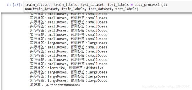
这里，我K值设置的默认值，为10。运气比较好，预测的分类效果还是可以。

---

值的注意的是，numpy的填充函数，即：np.tile(A, reps)，如：

np.tile(np.max(feature_dataset, axis=0), (feature_dataset.shape[0], 1)) - feature_dataset

A是重复的基元素，reps是重复填充的一个维度数组，原话是这么介绍的：The number of repetitions ofAalong each axis.，也就是可以按照x和y轴来进行重复多少次的填充。