matlab学习笔记-绘图

基础绘图

• matlab无法直接根据函数表达式画图；
• 先生成数值点，再根据数据绘图。

plot()

plot(x,y)：画出每个点(x,y)
plot(y)：画出每个点（x=[1…n],n=length(y)）
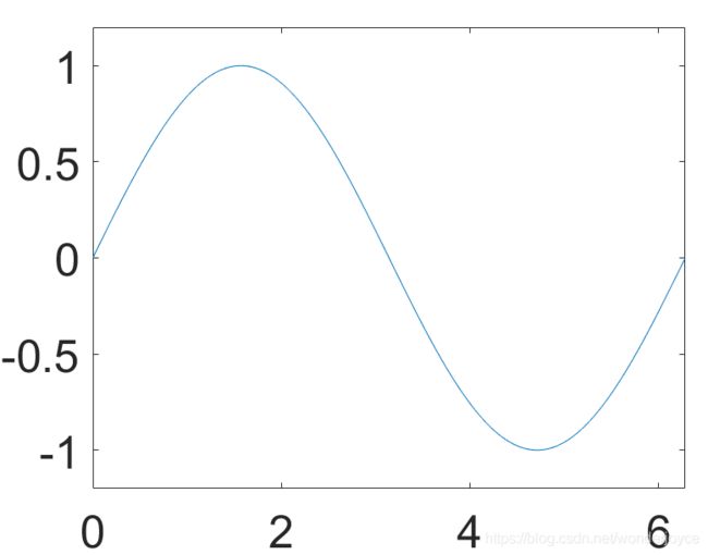
Example:

>> plot(cos(0:pi/20:2*pi))

同时保留多个图形

matlab会自动覆盖上一个图形，如果需要保留多个图形，需要用到hold on指令。

>> hold on
>> plot(cos(0:pi/20:2*pi));
>> plot(sin(0:pi/20:2*pi));
>> hold off

也可以先给变量和函数赋值，再一起使用plot绘图

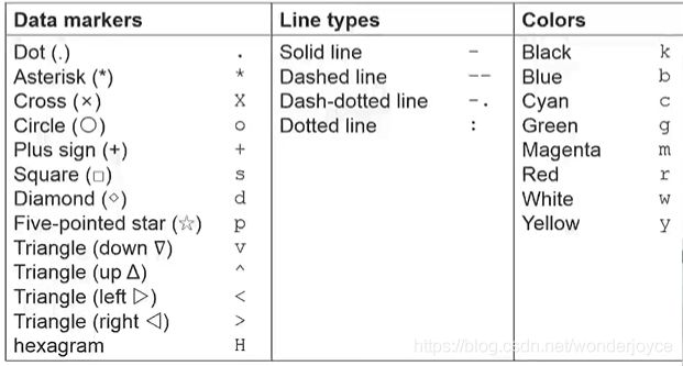
plot style 格式设定

plot(x,y,'str')：使用字符串对应的格式来绘图，详见下表

legend()

在图形中加入图例：

Legend('L1',...)

>> x=0:0.5:4*pi;
>> y=sin(x); h=cos(x); w=1./(1+exp(-x));
>> g=(1/(2*pi*2)^0.5).*exp((-1.*(x-2*pi).^2)./(2*2^2));
>> plot(x,y,'bd-',x,h,'gp:',x,g,'c^-',x,w,'ro-')
>> legend('sin(x)','cos(x)','Guass Function','Sigmoid')

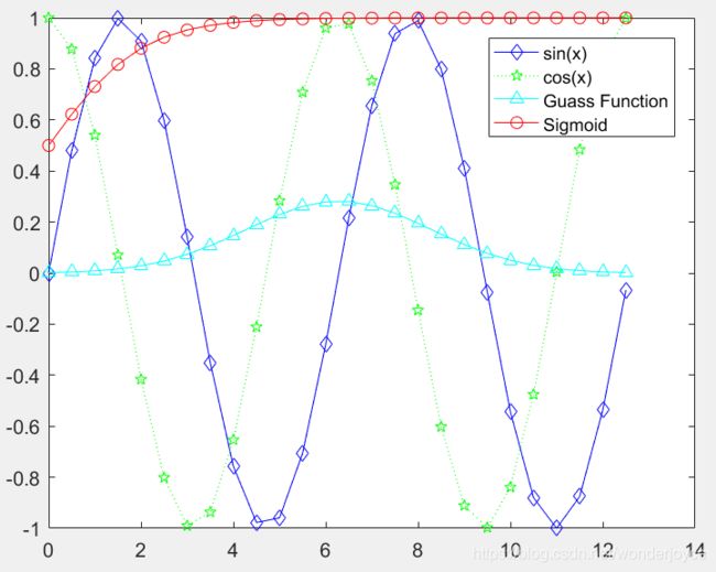
注：在legend()中添加‘Location’,'方位名'可以改变图例的位置

添加title或坐标轴名称

• title()
• xlabel()
• ylabel()
• zlabel()

>> x=0:0.1:2*pi;y1=sin(x);y2=exp(-x);
>> plot(x,y1,'--*',x,y2,':o');
>> xlabel('x= 0 to 2\pi');
>> ylabel('Values of sin(x) and e^{-x}');
>> title('Fuction plots of sin(x) and e^{-x}');
>> legend('sin(x)','e^{-x}');

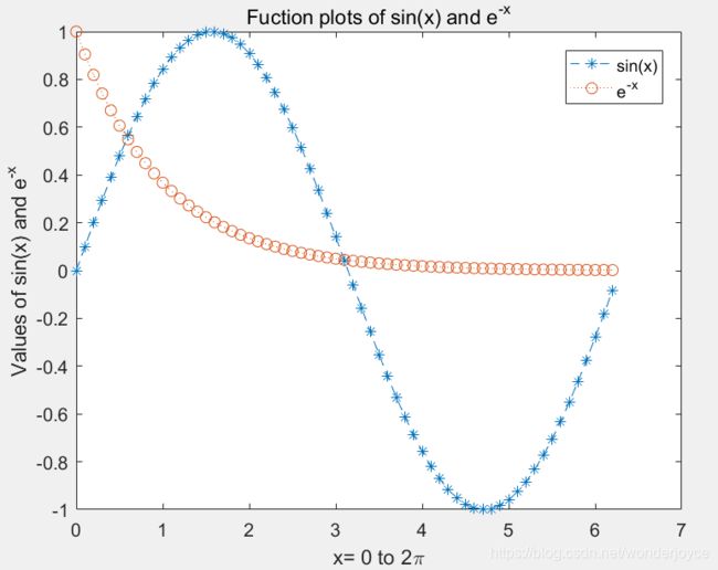
注：

• \pi 代表字符pai的意思，显示为π；
• 当指数为一串字符时，用{}括起来
  （此处实为latex语法）

text() & annotation()

• text()函数用来给图加上说明性文字。
  格式：text(x,y,'txt')
  或者：text(x,y,'txt','color','k')

• 用latex语法来显示字符串内容

text(x,y,'txt','Interpreter','latex')

>> x=linspace(0,3); y=x.^2.*sin(x); plot(x,y);
>> line([2,2],[0,2^2*sin(2)]);
>> str='$$\int_{0}^{2} x^2\sin(x) dx $$';
>> text(0.25,2.5,str,'Interpreter','latex');
>> annotation('arrow','X',[0.32,0.5],'Y',[0.6,0.4]);

• annotation()用来给图加上箭头或标注

语法	用途
annotation(annotation_type)	以指定的对象类型，使用默认属性值建立注释对象
annotation(‘line’,x,y)	建立从(x(1), y(1))到(x(2), y(2))的线注释对象。
annotation(‘arrow’,x,y)	建立从(x(1), y(1))到(x(2), y(2))的箭头注释对象。
annotation(‘doublearrow’,x,y)	建立从(x(1), y(1))到(x(2), y(2))的双箭头注释对象
annotation(‘textarrow’,x,y)	建立从(x(1),y(1))到(x(2),y(2))的带文本框的箭头注释对象。
annotation(‘ellipse’,[x y w h])	建立椭圆形注释对象。
annotation(‘rectangle’,[x y w h])	建立矩形注释对象。

注：这里的x,y指的是占整个图形的比例，而非对应坐标轴的具体值。

• Exercise：

t=linspace(1,2); f=t.^2; g=sin(2*pi.*t);
plot(t,f,'-k',t,g,'or');
xlabel('Time(ms)'); ylabel('f(t)');title('Mini assignment#1');
legend('t^{2}','sin(2\pit)','Location','northwest');

修改图形属性

包括图形、线条、tick等元素，此处与origin类似，进入编辑器需要修改哪里就点击哪里。

以下为通过指令来修改具体属性，使用时需要注意区分不同的对象。

1. 定义对象的辨识码（handle）

>> x=linspace(0,2*pi,1000); y=sin(x);
>> plot(x,y); set(gcf,'Color',[1,1,1]);
>> h=plot(x,y);

得到（x,y）线条的辨识码h。

• 相关效用函数：

函数名	用途
gca	返回现有坐标轴的指针
gcf	返回现有图形的指针
allchild	找到指定对象的所有子级
ancestor	找到图形对象的父级
delete	删除一个对象
findall	找到所有图形对象

2. 得到对象的属性：get()

>> h=plot(x,y);
>> get(h)
    AlignVertexCenters: 'off'
            Annotation: [1x1 matlab.graphics.eventdata.Annotation]
          BeingDeleted: 'off'
            BusyAction: 'queue'
         ButtonDownFcn: ''
              Children: [0x0 GraphicsPlaceholder]
              Clipping: 'on'
                 Color: [0 0.4470 0.7410]
            %后续省略

3. 修改该对象的属性

>> set(gca,'XLim',[0,2*pi]);
>> set(gca,'YLim',[-1.2,1.2]);

Before:

After: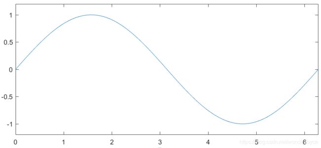

更改字号大小

set(gca,'FontSize',25);

修改坐标轴tickname

>>set(gca,'XTick',0:pi/2:2*pi);
>>set(gca,'XTickLabel',0:90:360);
>> set(gca,'XTickLabel',{
     '0','\pi/2','3\pi/2','2\pi'});

修改线条属性

>> set(h,'LineStyle','-.','Linewidth',7.0,'Color','g');

h应在修改各项属性之前定义好，否则会重新绘图覆盖之前的设置。

删除绘制的图线

delete(h);

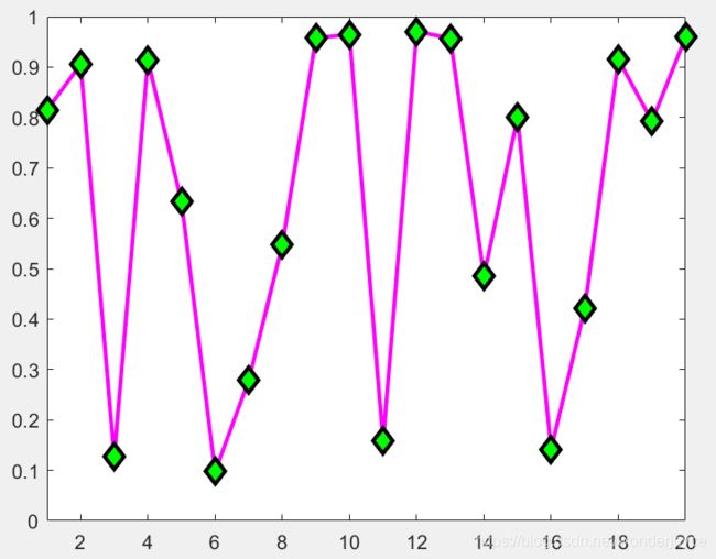
Marker的设置

>> x=rand(20,1);
>> set(gca,'FontSize',18);
>> plot(x,'-md','LineWidth',2,'MarkerEdgeColor','k','MarkerFaceColor','g','MarkerSize',10);
>> xlim([1,20]);

可以分别设置marker边缘和内里的颜色以及其大小。

多个图形的绘制

当存在多个图形时，要谨慎使用gcf这样的效用函数，只会指向现在新有的图形。

Figure生成位置的制定

figure('Position',[left,bottom,width,height]);

在一张大图上集成多张小图

subplot(m.n,1);

>> t=0:0.1:2*pi;x=3*cos(t); y=sin(t);
>> subplot(2,2,1);plot(x,y);axis normal;
>> subplot(2,2,2);plot(x,y);axis square;
>> subplot(2,2,3);plot(x,y);axis equal;
>> subplot(2,2,4);plot(x,y);axis equal tight;

Grid、Box、Axis常用指令

指令	用途
grid on/off	显示或隐藏坐标区网格线
box on/off	显示或隐藏坐标区轮廓
axis on/off	显示或隐藏坐标轴
axis normal	还原默认行为。
axis equal	沿每个坐标轴使用相同的数据单位长度。
axis square	使用相同长度的坐标轴线。相应调整数据单位之间的增量。
axis equal tight	将坐标轴范围设置为等同于数据范围，使轴框紧密围绕数据。
axis image	沿每个坐标区使用相同的数据单位长度，并使坐标区框紧密围绕数据。
axis ij	反转方向。对于二维视图中的坐标区，y 轴是垂直的，值从上到下逐渐增加。
axis xy	默认方向。对于二维视图中的坐标区，y 轴是垂直的，值从下到上逐渐增加。

把画好的图形保存为成文件

saveas(gcf,'','');

例如：

• 保存为png格式：

saveas(gcf,'Barchart.png')

• 保存为png格式：

saveas(gcf,'Barchart','epsc')

如果需要保存为更高分辨率的格式，需要用到print指令，详见： print帮助链接

进阶2D绘图

对数图

命令	用途
semilogx	按照 x 轴的对数刻度绘制数据
semilogy	按照 y 轴的对数刻度绘制数据
loglog	使用 x 轴和 y 轴的对数刻度创建绘图

例:

>> x=logspace(-1,1,100);
>> y=x.^2;
>> subplot(2,2,1); plot(x,y); title('Plot');
>> subplot(2,2,2); semilogx(x,y); title('Semilogx');
>> subplot(2,2,3); semilogy(x,y); title('Semilogy');
>> subplot(2,2,4); loglog(x,y); title('Loglog');

加上网格：

grid on;
%或者
set(gca,'xGrid','on');

创建具有两个 y 轴的图形

plotyy（）

更推荐使用：

yyaxis left
yyaxis right

例：

>> x=0:0.01:20;
>> y1=200*exp(-0.05*x).*sin(x);
>> y2=0.8*exp(-0.5*x).*sin(10*x);
>> yyaxis left
>> plot(x,y1); ylabel('Left Y-Axis');
>> yyaxis right
>> plot(x,y2); ylabel('Right Y-Axis');
>> title('振荡衰减')；

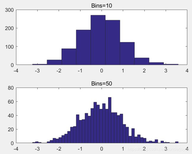
直方图

直方图属于数值数据的条形图类型，将数据分组为 bin。

>> y=randn(1,1000);
>> subplot(2,1,1); hist(y,10); title('Bins=10');
>> subplot(2,1,2); hist(y,50); title('Bins=50');

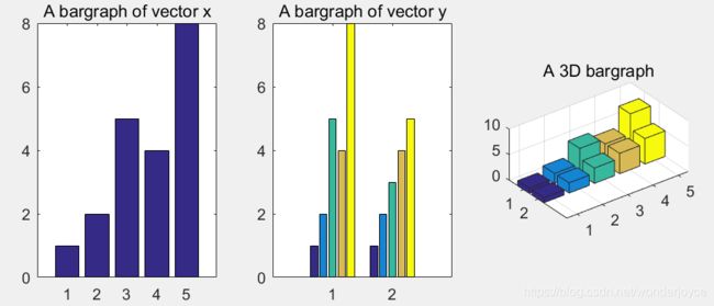
条形图

创建一个条形图，y 中的每个元素对应一个条形。如果 y 是 m×n 矩阵，则 bar 创建每组包含 n 个条形的 m 个组。

>> x=[1,2,5,4,8];y=[x;1:5];
>> subplot(1,3,1); bar(x); title('A bargraph of vector x');
>> subplot(1,3,2); bar(y); title('A bargraph of vector y');
>> subplot(1,3,3); bar3(y); title('A 3D bargraph');

堆叠&水平排列式条形图：

>> x=[1,2,5,4,8];y=[x;1:5];
>> subplot(1,2,1);bar(y,'stacked');title('stacked');
>> subplot(1,2,2);barh(y);title('horizontal');

扇形图

>> a=[10 5 20 30];
>> subplot(1,3,1); pie(a);
>> subplot(1,3,2); pie(a,[0,0,0,1]);
>> subplot(1,3,3); pie3(a,[0,0,0,1]);

极坐标图

>> x=1:100; theta=x/10; r=log10(x);
>> subplot(1,4,1); polar(theta,r);
>> theta=linspace(0,2*pi); r=cos(4*theta);
>> subplot(1,4,2); polar(theta,r);
>> theta=linspace(0,2*pi,6); r=ones(1,length(theta));
>> subplot(1,4,3); polar(theta,r);
>> theta=linspace(0,2*pi); r=1-sin(theta);
>> subplot(1,4,4); polar(theta,r);

注：极坐标图可以用来绘制正多边形，非常简便：
绘制正n边形：

>> theta=linspace(0,2*pi,n+1); r=ones(1,length(theta));
>> polar(theta,r);

如n=6时，得到：

阶梯图&针状图

>> x=linspace(0,4*pi,40); y=sin(x);
>> subplot(1,2,1); stairs(y);
>> subplot(1,2,2); stem(y);

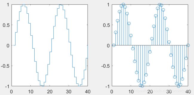
stem可用来添加标记点，如不需要竖线，可在绘制时设置（‘LineStyle’,'none'）。

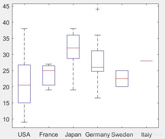
箱线图&含误差条的线图

>> load carsmall
>> boxplot(MPG,Origin);

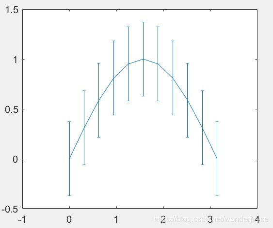
>> x=0:pi/10:pi;
>> y=sin(x);
>> e=std(y)*ones(size(x));
>> errorbar(x,y,e);

Fill() 给封闭图形上色

>> t=(1:2:15)'*pi/8;
>> x=sin(t); y=cos(t);
>> fill(x,y,'r');
>> axis square off;
>> text(0,0,'STOP','Color','w','FontSize',80,...
'FontWeight','bold','HorizontalAlignment','Center');

>> t=linspace(0,2*pi,5);
>>x=sin(t); y=cos(t);
>>fill(x,y,'y','LineWidth',5);
>>axis square off
>>text(0,0,'WAIT','Color','k','FontSize',76,...
'FontWeight','bold','HorizontalAlignment','Center');

色彩配置

颜色的指定方式

用 [R G B] 向量来决定颜色。
需要把常规使用的0~ 255，等比转化为0~1。

>> G=[46 38 29 24 13];
>> S=[29 27 17 26 8];
>> B=[29 23 19 32 7];
>> h=bar(1:5,[G' S' B']);
>> title('Medal count for top 5 countries in 2012 Olympics');
>> ylabel('Number of Medals'); xlabel('Country');
>> legend('Gold','Silver','Bronze');
>> set(gca,'XTickLabel',{
     'USA','CHN','GBR','RUS','KOR'});
>> set(h(1),'FaceColor',[1,0.8431,0]);
>>set(h(2),'FaceColor',[0.7529,0.7529,0.7529]);
>>set(h(3),'FaceColor',[0.7490,0.6784,0.4353]);

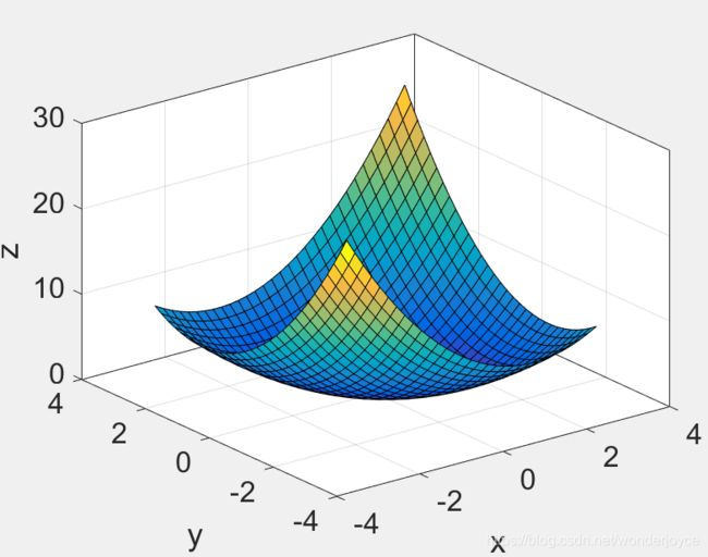
imagesc() 用颜色表示数值

显示使用经过标度映射的颜色的图像.

>> [x,y]=meshgrid(-3:.2:3,-3:.2:3);
>> z=x.^2+x.*y+y.^2;
>> surf(x,y,z);
>> box on;
>> set(gca,'FontSize',16); zlabel('z');
>> xlim([-4,4]); xlabel('x');
>> ylim([-4,4]); ylabel('y');
>> imagesc(z); 
>> axis square
>> xlabel('x');ylabel('y');

Before:

After:

加上colorbar:
>> colorbar;

colormap

• matlab有很多内置的colormap，可以直接调用。

colormap([name]);

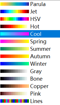
• 每一个colormap都是一个256*3的矩阵。

a=colormap(prism);

• 可以使用自己定义的colormap:

>> a=ones(256,3);
>> colormap(a);

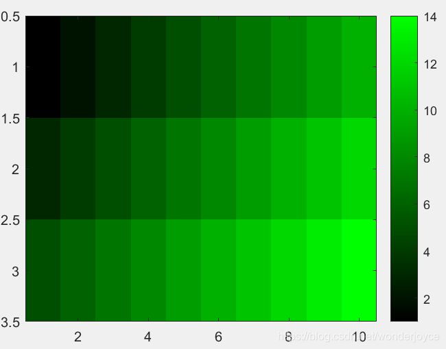
例：生成一个全绿的colormap

>> Green=zeros(256,3);
>> Green(:,2)=linspace(0,1,256)';
>> x=[1:10;3:12;5:14];
>> imagesc(x);
>> colormap(Green);
>> colorbar;

3D绘图

几个重要指令

指令	用途
plot3	绘制三维空间中的坐标
surf	创建一个三维曲面图
surfc	创建一个三维曲面图，其下方有等高线图
surface	创建一个基本三维曲面图。该函数将矩阵 Z 中的值绘制为由 X 和 Y 定义的 x-y 平面中的网格上方的高度
mesh	网格曲面图
meshc	网格曲面图下的等高线图
contour	矩阵的等高线图
contourf	填充的二维等高线图

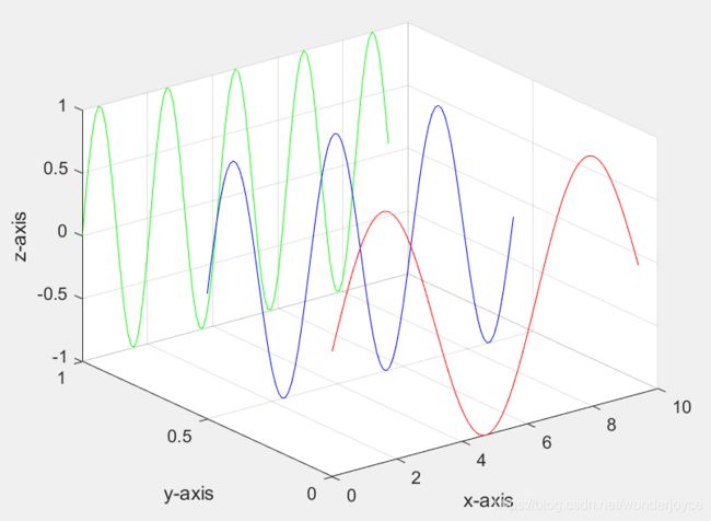
plot3()

>> x=0:0.1:3*pi;
>> z1=sin(x); z2=sin(2*x); z3=sin(3*x);
>> y1=zeros(size(x)); y3=ones(size(x));
>> y2=y3./2;
>> plot3(x,y1,z1,'r',x,y2,z2,'b',x,y3,z3,'g');
>> grid on;
>> xlabel('x-axis'); ylabel('y-axis'); zlabel('z-axis');

其他更多3D图形：

>> t=0:pi/50:10*pi;
>> plot3(sin(t),cos(t),t);
>> grid on
>> axis square;

>> turns=40*pi;
>> t=linspace(0,turns,4000);
>> x=cos(t).*(turns-t)./turns;
>> y=sin(t).*(turns-t)./turns;
>> z=t./turns;
>> plot3(x,y,z); grid on;

3D曲面图

• 此时通常z是x和y的函数，即:z=f(x,y);
• 使用meshgrid创建一个基于向量 x 和 y 中包含的坐标返回的二维网格坐标。

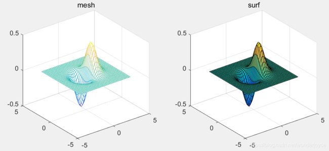
对比mesh()和surf()

>> x=-3.5:0.2:3.5;
>> y=-3.5:0.2:3.5;
>> [X,Y]=meshgrid(x,y);
>> Z=X.*exp(-X.^2-Y.^2);
>> subplot(1,2,1); mesh(X,Y,Z);
>> subplot(1,2,2); surf(X,Y,Z);

contour()

等高线图，类似上面图形的顶面投影。

>> subplot(2,1,1); mesh(X,Y,Z);title('mesh');axis square;
>> subplot(2,1,2); contour(X,Y,Z);title('contour');axis square;

不同的contour图：

>> subplot(1,3,1); contour(Z,[-.45:.05:.45]);title('在指定位置显示等高线');axis square;
>> subplot(1,3,2); [C,h]=contour(Z); clabel(C,h);title('更改属性：有标识');axis square;
>> subplot(1,3,3); contourf(Z); ;title('填充的等高线图');axis square;

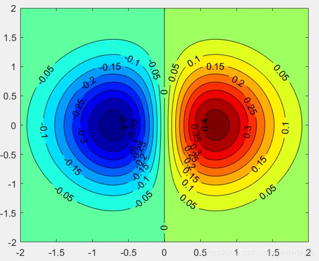
小练习：

>> x=-2.0:0.01:2.0; y=-2.0:0.01:2.0;
>> [X,Y]=meshgrid(x,y);
>> Z=X.*exp(-X.^2-Y.^2);
>> [C,h]=contourf(X,Y,Z,[-.45:.05:.45]);
>> clabel(C,h);
>> colormap(jet);

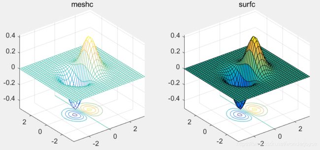
meshc()和surfc()

在原有基础上增加了等高线的投影：

>> subplot(1,2,1); meshc(X,Y,Z);title('meshc');
>> subplot(1,2,2); surfc(X,Y,Z);title('surfc');

观察角度 view()

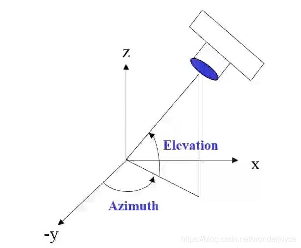
设定观察角度：view(-45,20);

>> sphere(50); shading flat;
>> light('Position',[1 3 2]);
>> light('Position',[-3 -1 3]);
>> material shiny;
>> axis vis3d off;
>> set(gcf,'Color',[1 1 1]);
>> view(-45,20);

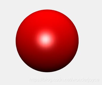
光线 light()

>> [X,Y,Z]=sphere(64); h=surf(X,Y,Z);
>> axis square vis3d off;
>> reds=zeros(256,3); reds(:,1)=linspace(0,1,256);
>> colormap(reds); 
>> shading interp;
>> lighting phong;
>> set(h,'AmbientStrength',0.75,'DiffuseStrength',0.5);
>> L1=light('Position',[-1,-1,-1]);

可以调整灯光的位置：

>> set(L1,'Position',[-1,-1,1]);

可以调整灯光的颜色：

>> set(L1,'Color','g');

patch()

用来绘制一个或多个填充多边形区域。
设定好多边形每条边的向量。

>> v=[0 0 0;1 0 0;1 1 0;0 1 0;0.25 0.25 1;...
      0.75 0.25 1;0.75 0.75 1;0.25 0.75 1];
>> f=[1 2 3 4;5 6 7 8;1 2 6 5;2 3 7 6;3 4 8 7;4 1 5 8];
>> subplot(1,2,1);patch('Vertices',v,'Faces',f,'FaceVertexCData',hsv(6),'Facecolor','flat');
>> view(3);
>> axis square tight; grid on;
>> subplot(1,2,2);patch('Vertices',v,'Faces',f,'FaceVertexCData',hsv(8),'Facecolor','interp');
>> view(3);
>> axis square tight; grid on;