loam论文翻译

Abstract

We propose a real-time method for odometry and mapping using range measurements from a 2-axis lidar moving in 6-DOF . The problem is hard because the range measurements are received at different times, and errors in motion estimation can cause mis-registration of the resulting point cloud. To date, coherent 3D maps can be built by off-line batch methods, often using loop closure to correct for drift over time. Our method achieves both low-drift and low-computational complexity without the need for high accuracy ranging or inertial measurements. The key idea in obtaining this level of performance is the division of the complex problem of simultaneous localization and mapping, which seeks to optimize a large number of variables simultaneously, by two algorithms. One algorithm performs odometry at a high frequency but low fidelity to estimate velocity of the lidar. Another algorithm runs at a frequency of an order of magnitude lower for fine matching and registration of the point cloud. Combination of the two algorithms allows the method to map in real-time. The method has been evaluated by a large set of experiments as well as on the KITTI odometry benchmark. The results indicate that the method can achieve accuracy at the level of state of the art offline batch methods.
我们提出了一种在6自由度范围内利用2轴激光雷达进行距离测量实现SLAM的方法。这个问题难点在于 测量的距离信息是在不同的时间接收的（因为激光雷达需要通过旋转的方式采集信息），运动估计中的误差可能会导致最终点云的错误配准。迄今为止，通过off-line batch方法可以构建3D地图，并使用loop closure来校正随时间的漂移。我们实现了一种低漂移和低计算复杂度的方法，无需高精度测距或惯性测量。该方法的核心思路是通过两种算法来实现分别定位和建图的问题，我们的方法可以同时优化大量变量。第一个算法以高频但低精度的性能进行里程计测量，以估计激光雷达的速度。第二个算法以较低数量级的频率运行，用于点云的精细匹配和对齐（registation）（类似于SLAM中的前端和后端）。通过两种算法的结合允许该方法实时建图。该方法已通过大量实验以及KITTI里程计基准进行了评估。结果表明，该方法可以达到off-line batch处理方法的精度水平。

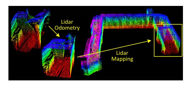
Fig. 1. The method aims at motion estimation and mapping using a moving 2-axis lidar. Since the laser points are received at different times, distortion is present in the point cloud due to motion of the lidar (shown in the left lidar cloud). Our proposed method decomposes the problem by two algorithms running in parallel. An odometry algorithm estimates velocity of the lidar and corrects distortion in the point cloud, then, a mapping algorithm matches and registers the point cloud to create a map. Combination of the two algorithms ensures feasibility of the problem to be solved in real-time.
图1所示。该方法利用移动的2轴激光雷达进行运动估计和建图。由于激光雷达的运动，激光点是在不同的时间接收到的，在点云中会出现失真(如图左激光雷达云所示)。我们提出的方法通过两个并行的算法来分解问题。一种odometry算法估计激光雷达的速度并校正点云中的失真，然后一种mapping算法匹配并对齐（registers）点云来创建地图。两种算法的结合保证了所要解决问题的实时性。

I. INTRODUCTION

3D mapping remains a popular technology [1]–[3]. Mapping with lidars is common as lidars can provide high frequency range measurements where errors are relatively constant irrespective of the distances measured. In the case that the only motion of the lidar is to rotate a laser beam, registration of the point cloud is simple. However, if the lidar itself is moving as in many applications of interest, accurate mapping requires knowledge of the lidar pose during continuous laser ranging. One common way to solve the problem is using independent position estimation (e.g. by a GPS/INS) to register the laser points into a fixed coordinate system. Another set of methods use odometry measurements such as from wheel encoders or visual odometry systems [4], [5] to register the laser points. Since odometry integrates small incremental motions over time, it is bound to drift and much attention is devoted to reduction of the drift (e.g. using loop closure).
3D建图仍然是一种主流的技术[1]–[3]。使用激光雷达进行建图是非常 常见的，因为激光雷达可以提供高频的距离测量信息，无论测量的距离如何，误差都相对恒定。当激光雷达的唯一运动是旋转激光束时，其点云的配准非常简单。然而，如果激光雷达（多自由度运动）in many applications of interest中运动，则精确的测绘需要在连续激光测距期间了解激光雷达的姿态变换。解决该问题的一种常见方法是使用独立的位置估计（例如通过GPS/INS）将激光点对齐到固定的坐标系中。另一组方法使用里程计测量，例如从车轮编码器或视觉里程计系统[4]，[5]记录激光点。由于里程计集成了随时间推移的小增量运动，因此必然会发生漂移，并且会将大量注意力放在减小漂移上（例如，使用loop closure）。

Here we consider the case of creating maps with lowdrift odometry using a 2-axis lidar moving in 6-DOF. A key advantage of using a lidar is its insensitivity to ambient lighting and optical texture in the scene. Recent developments in lidars have reduced their size and weight. The lidars can be held by a person who traverses an environment [6], or even attached to a micro aerial vehicle [7]. Since our method is intended to push issues related to minimizing drift in odometry estimation, it currently does not involve loop closure.
在这里，我们考虑使用在6自由度运动的2轴激光雷达进行地图创建的场景。使用激光雷达的一个关键优势是它对场景中的环境光明和光学纹理不敏感。激光雷达的最新发展缩小了它们的尺寸和重量。激光雷达可以由人手持[6]，甚至可以连接到微型飞行器[7]。由于我们的方法旨在推动里程计估计中的最小化dift的问题，因此目前不涉及loop closure。

The method achieves both low-drift and low-computational complexity without the need for high accuracy ranging or inertial measurements. The key idea in obtaining this level of performance is the division of the typically complex problem of simultaneous localization and mapping (SLAM) [8], which seeks to optimize a large number of variables simultaneously, by two algorithms. One algorithm performs odometry at a high frequency but low fidelity to estimate velocity of the lidar. Another algorithm runs at a frequency of an order of magnitude lower for fine matching and registration of the point cloud. Although unnecessary, if an IMU is available, a motion prior can be provided to help account for high frequency motion. Specifically, both algorithms extract feature points located on sharp edges and planar surfaces, and match the feature points to edge line segments and planar surface patches, respectively. In the odometry algorithm, correspondences of the feature points are found by ensuring fast computation. In the mapping algorithm, the correspondences are determined by examining geometric distributions of local point clusters, through the associated eigenvalues and eigenvectors.
该方法实现了低漂移和低计算复杂度，无需高精度测距或惯性测量。获得这一性能水平的关键思想是通过两种算法将SLAM[8]进行划分，该问题寻求（seek）同时优化大量变量。一种算法以高频但低精度的性能进行里程测量，以估计激光雷达的速度。另一种算法以较低数量级的频率运行，用于点云的精细匹配和对齐（registration）。尽管非必要，但如果IMU可用，则可以用于提供运动先验以帮助计算高频运动。具体来说，这两种算法都提取位于锐边和平面上（sharp edges and planar surfaces）的特征点，并分别将特征点与边线段和平面匹配。在里程计算法中，通过足够快速的计算来找到特征点的对应关系。在mapping算法中，通过相关的特征值和特征向量检查局部点簇（local point clusters） 的几何分布来确定对应关系。

By decomposing the original problem, an easier problem is solved first as online motion estimation. After which, mapping is conducted as batch optimization (similar to iterative closest point (ICP) methods [9]) to produce high-precision motion estimates and maps. The parallel algorithm structure ensures feasibility of the problem to be solved in real-time. Further, since the motion estimation is conducted at a higher frequency, the mapping is given plenty of time to enforce accuracy. When running at a lower frequency, the mapping algorithm is able to incorporate a large number of feature points and use sufficiently many iterations for convergence.
通过对原始问题进行分解，首先解决了一个简单的问题，即在线运动估计。之后，mapping作为批量优化（类似于迭代最近点（ICP）方法[9]）进行，以生成高精度运动估计和maps。并行算法结构保证了问题实时求解的可行性。此外，由于运动估计是在更高的频率下进行的，因此给了mapping足够的时间来提高精度。当以较低的频率运行时，mapping算法能够包含大量的特征点，并使用足够多的迭代进行收敛。

II .Related work

III. Notation and Task Description（符号和任务描述）

The problem addressed in this paper is to perform ego-motion estimation with point cloud perceived by a 3D lidar, and build a map for the traversed environment. We assume that the lidar is pre-calibrated. We also assume that the angular and linear velocities of the lidar are smooth and continuous over time, without abrupt changes. The second assumption will be released by usage of an IMU, in Section VII-B.
本文解决的问题是利用三维激光雷达感知到的点云进行自运动估计，并建立遍历环境的地图。我们假设激光雷达是预先校准的。我们还假设激光雷达的角速度和线速度是平滑和连续的，没有突变。第二项假设将在Section VII-B中通过使用IMU提出。

As a convention in this paper, we use right uppercase superscription to indicate the coordinate systems. We define a sweep as the lidar completes one time of scan coverage. We use right subscription $k,k\in Z^{+}$to indicate the sweeps, and $P_k$ to indicate the point cloud perceived during sweep k. Let us define two coordinate systems as follows.
我们使用右上角的大写上标来表示坐标系。我们将扫描定义为激光雷达完成一次扫描覆盖 。我们使用右下角的小写下标 $k,k\in Z+$表示扫描， $P_k$ 表示第$k$次扫描期间感知到的点云。让我们定义如下两个坐标系。

•Lidar coordinate system $L$ is a 3D coordinate system with its origin at the geometric center of the lidar. The x-axis is pointing to the left, the y-axis is pointing upward, and the z-axis is pointing forward. The coordinates of a point $i,i\in P_k$, in$L_k$ are denoted as $X_{(k,i)}^L$.
•World coordinate system $W$ is a 3D coordinate system coinciding with$L$ at the initial position. The coordinates of a point $i,i\in P_k$, in $W_k$are $X_{(k,i)}^W$
•激光雷达坐标系$L$是一个三维坐标系，其原点位于激光雷达的几何中心。x轴指向左侧，y轴指向上方，z轴指向前方。激光点$i，i\in P_k$在$L_k$坐标系下表示为$X_{(k,i)}^L$。
•世界坐标系$W$是一个3D坐标系，在初始位置与$L$重合。激光点$i，i\in P_k$ 在 $W_k$ 坐标系下表示为$X_{(k,i)}^W$

With assumptions and notations made, our lidar odometry and mapping problem can be defined as
通过假设和标记，我们的激光雷达里程测量和mapping问题可以定义为

Problem: Given a sequence of lidar cloud$P_k,k\in Z^{+}$, compute the ego-motion of the lidar during each sweepk, and build a map with $P_k$ for the traversed environment.
问题: 给定一个激光点云序列$P_k,k\in Z^{+}$，计算每次扫描时激光雷达的自运动，用 $P_k$构建遍历环境的地图。

IV. System Overview

A. Lidar Hardware

The study of this paper is validated on, but not limited to a custom built 3D lidar based on a Hokuyo UTM-30LX laser scanner. Through the paper, we will use data collected from the lidar to illustrate the method. The laser scanner has a field of view of 180◦with 0.25◦ resolution and 40 lines/sec scan rate. The laser scanner is connected to a motor, which is controlled to rotate at an angular speed of180◦/s between −90◦ and 90◦ with the horizontal orientation of the laser scanner as zero. With this particular unit, a sweep is a rotation from −90◦ to 90◦ or in the inverse direction (lasting for 1s). Here, note that for a continuous spinning lidar, a sweep is simply a semispherical rotation. An onboard encoder measures the motor rotation angle with a resolution of 0.25◦, with which, the laser points are projected into the lidar coordinates,$L$.
本文的研究在基于Hokuyo UTM-30LX激光扫描仪的定制3D激光雷达上得到验证，但不限于此。通过本文，我们将使用从激光雷达收集的数据来说明该方法。激光扫描仪的视场为180度,分辨率为0.25度，扫描速率为40行/秒。激光扫描仪与电机相连，电机被控制以180度/s (−90◦到90◦)的角速度旋转,激光扫描仪的水平角度为零。对于此特定单元，扫描是从−90◦到90◦或相反方向进行的（持续1s）。请注意，对于连续旋转的激光雷达，扫描只是一个半球形旋转。车载编码器以0.25度的分辨率测量电机旋转角度, 激光点被投影到激光雷达坐标$L$。

B. Software System Overview

Fig. 3 shows a diagram of the software system. Let $\hat{P}$ be the points received in a laser scan. During each sweep,$\hat{P}$ is registered in{L}. The combined point cloud during sweep k forms $P_k$. Then,$P_k$ is processed in two algorithms. The lidar odometry takes the point cloud and computes the motion of the lidar between two consecutive sweeps. The estimated motion is used to correct distortion in $P_k$. The algorithm runs at a frequency around 10Hz. The outputs are further processed by lidar mapping, which matches and registers the undistorted cloud onto a map at a frequency of 1Hz. Finally, the pose transforms published by the two algorithms are integrated to generate a transform output around 10Hz, regarding the lidar pose with respect to the map. Section V and VI present the blocks in the software diagram in detail.
图3为软件系统框图。定义 $\hat{P}$ 为激光扫描收到的点。在每次扫描期间，$\hat{P}$ 在 激光雷达坐标系 $L$ 中对齐。第k次扫描期间的点云组合形成$P_k$。然后，用两种算法处理$P_k$。激光雷达里程计通过点云，计算激光雷达在两次连续扫描之间的运动。估计的运动被用来校正在$P_k$中的畸变。该算法的运行频率约为10Hz。输出的结果被激光雷达mapping算法施行进一步的处理，它以1Hz的频率将去畸变的点云匹配并对齐到地图上。最后，将两种算法发布的姿态变换进行集成，得到激光雷达姿态相对于地图的约10Hz的变换输出。Section V and VI 对软件框图中的模块进行了详细介绍。

V. Lidar Odometry

A. Feature Point Extraction

We start with extraction of feature points from the lidar cloud,$P_k$. The lidar presented in Fig. 2 naturally generates unevenly distributed points inPk. The returns from the laser scanner has a resolution of0.25◦within a scan. These points are located on a scan plane. However, as the laser scanner rotates at an angular speed of 180◦/s and generates scans at 40Hz, the resolution in the perpendicular direction to the scan planes is 180◦/40 = 4.5◦. Considering this fact, the feature points are extracted from $P_k$ using only information from individual scans, with co-planar geometric relationship.
我们首先从激光雷达云$P_k$中提取特征点。图2所示的激光雷达在$P_k$中会产生分布不均匀的点。激光扫描仪返回的分辨率为0.25◦。这些点位于一个扫描平面上。但是，由于激光扫描仪以180◦/s的角速度旋转并以40Hz的频率生成扫描，垂直于扫描平面的分辨率为180◦/40 = 4.5◦考虑到这一事实，从$P_k$中提取的特征点，仅使用单个扫描的信息，具有共面几何关系.

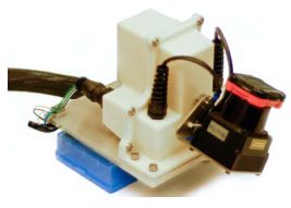
Fig. 2. The 3D lidar used in this study consists of a Hokuyo laser scanner driven by a motor for rotational motion, and an encoder that measures the rotation angle. The laser scanner has a field of view of180◦with a resolution of0.25◦. The scan rate is 40 lines/sec. The motor is controlled to rotate from −90◦to90◦with the horizontal orientation of the laser scanner as zero.
图2所示。本研究使用的3D激光雷达由一个旋转运动电机驱动的Hokuyo激光扫描仪和一个测量旋转角度的编码器组成。激光扫描仪的视场为180◦分辨率为0.25◦。扫描速度为40行/秒。电机被控制为从−90◦到90◦的旋转，且水平方向上角度为零。

We select feature points that are on sharp edges and planar surface patches. Let $i$ be a point in $P_k$ ,i∈ $P_k$, and let $S$ be the set of consecutive points of $i$ returned by the laser scanner in the same scan. Since the laser scanner generates point returns in CW or CCW order,$S$ contains half of its points on each side of $i$ and 0.25◦ intervals between two points. Define a term to evaluate the smoothness of the local surface,
我们选择位于锐边和平面 patches上的特征点（选择面点和角点作为特征点）。定义$i$为激光雷达点云$P_k$中的一个点，i∈ $P_k$，设$S$为激光扫描仪在同一次扫描中返回的$i$的连续点集。由于激光扫描仪以CW或CCW顺序（顺时针或逆时针）返回生成点，$S$在$i$ 和 0.25◦间隔的每一侧包含其点的一半。定义一个 term 以评估局部曲面的平滑度（曲率），

$j$ 就是在 $i$ 周围的点
曲率 = （当前点到其附近点的距离差 / 当前点的值 ) 的总和再求平均 = 平均的距离差

The points in a scan are sorted based on the $c$ values, then feature points are selected with the maximum $c$’s, namely, edge points, and the minimumc’s, namely planar points. To evenly distribute the feature points within the environment, we separate a scan into four identical subregions. Each subregion can provide maximally 2 edge points and 4 planar points. A point $i$ can be selected as an edge or a planar point only if its $c$ value is larger or smaller than a threshold, and the number of selected points does not exceed the maximum.
扫描中的点根据 $c$ 值（曲率）进行排序，然后选择具有最大 $c$ 值（即边缘点）和最小 $c$ 值（即平面点）的特征点。为了在环境中均匀分布特征点，我们将扫描分为四个相同的子区域（代码中是6等分）。每个子区域最多可提供2个边点和4个平面点。仅当点 $i$ 的 $c$ 值大于或小于阈值且所选点的数量不超过最大值时，才可以将点 $i$ 选择为边或平面点。

While selecting feature points, we want to avoid points whose surrounded points are selected, or points on local planar surfaces that are roughly parallel to the laser beams (pointB in Fig. 4(a)). These points are usually considered as unreliable. Also, we want to avoid points that are on boundary of occluded regions [23]. An example is shown in Fig. 4(b). PointA is an edge point in the lidar cloud because its connected surface (the dotted line segment) is blocked by another object. However, if the lidar moves to another point of view, the occluded region can change and become observable. To avoid the aforementioned points to be selected, we find again the set of points $S$. A point $i$ can be selected only if $S$ does not form a surface patch that is roughly parallel to the laser beam, and there is no point in $S$ that is disconnected from $i$ by a gap in the direction of the laser beam and is at the same time closer to the lidar then point $i$ (e.g. point $B$ cin Fig. 4(b))
在选择特征点时，我们希望避免选择其周围点已经被选择的点，或局部平面上与激光束大致平行的点（图4（a）中的点B）。这些点通常被认为是不可靠的。此外，我们还希望避免位于遮挡区域边界上的点[23]。图4（b）中示出了一个示例。Point A是激光雷达云中的一个边缘点，因为其连接表面（虚线段）被另一个对象阻挡。但是，如果激光雷达移动到另一个视角，则遮挡区域可能会发生变化并变得可见。为了避免选择上述点，我们再次找到点集$S$。仅当$S$未形成大致平行B于激光束的 surface patch，且$S$中没有任何点通过激光束方向上的间隙与$i$断开，同时更靠近激光雷达（如图4（b）中的点 B）时，才可选择点$i$

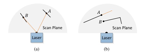
Fig. 4. (a) The solid line segments represent local surface patches. PointA is on a surface patch that has an angle to the laser beam (the dotted orange line segments). PointBis on a surface patch that is roughly parallel to the laser beam. We treat B as a unreliable laser return and do not select it as a feature point. (b) The solid line segments are observable objects to the laser. Point A is on the boundary of an occluded region (the dotted orange line segment), and can be detected as an edge point. However, if viewed from a different angle, the occluded region can change and become observable. We do not treatAas a salient edge point or select it as a feature point.
图4所示。(a)实线段表示local surface patches。Point A在一个surface patch上，它与激光束(橙色点线段)有一定的角度。point B位于一个与激光束大致平行的surface patch上。我们将B视为不可靠的激光回波，不选择它作为特征点。(b)实线段是激光的可观测对象。point A位于被遮挡区域(橙色点线段)的边界上，可以被检测为边缘点。然而，如果从不同的角度看，被遮挡的区域可以改变并变得可见。我们不把a作为一个显著的边缘点，也不把它作为一个特征点。

In summary, the feature points are selected as edge points starting from the maximum $c$ value, and planar points starting from the minimum $c$ value, and if a point is selected,
总之，特征点被选择为从最大$c$值开始的边点和从最小$c$值开始的平面点，如果一个点要被选择，

• The number of selected edge points or planar points cannot exceed the maximum of the subregion, and
• None of its surrounding point is already selected, and
• It cannot be on a surface patch that is roughly parallel to the laser beam, or on boundary of an occluded region.
• 选择的边缘点或平面点的数量不能超过子区域的最大值，并且
• 它的周围点都没有被选择，并且
• 它不能在大致平行于激光束的surface patch上，或位于封闭区域的边界。

An example of extracted feature points from a corridor scene is shown in Fig. 5. The edge points and planar points are labeled in yellow and red colors, respectively.
从走廊场景中提取特征点的实例如图5所示。边缘点和平面点分别用黄色和红色标注。

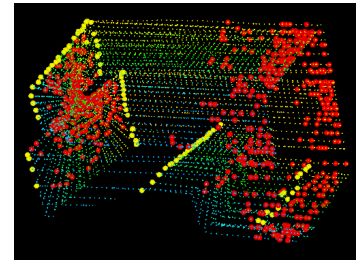
Fig. 5. An example of extracted edge points (yellow) and planar points (red) from lidar cloud taken in a corridor. Meanwhile, the lidar moves toward the wall on the left side of the figure at a speed of 0.5m/s, this results in motion distortion on the wall.
图5所示。从一条走廊的激光雷达云中提取边缘点(黄色)和平面点(红色)的例子。同时，激光雷达以0.5m/s的速度向图像左侧墙体移动，导致墙体运动变形。

B. Finding Feature Point Correspondence

The odometry algorithm estimates motion of the lidar within a sweep. Let $t_k$ be the starting time of a sweep $k$. At the end of each sweep, the point cloud perceived during the sweep,$P_k$, is reprojected to time stamp $t_{k+1}$, illustrated in Fig. 6. We denote the reprojected point cloud as${\overline{P}}_k$. During the next sweep $k+1$,${\overline{P}}_k$ is used together with the newly received point cloud,$P_{k+1}$, to estimate the motion of the lidar.
里程计算法估计激光雷达在扫描范围内的运动。让$t_k$作为扫描$k$的开始时间。在每次扫描结束时，扫描期间感知到的点云$P_k$被重新投影到时间戳$t_{k+1}$，如图6所示。我们将重新投影的点云表示为${\overline{P}}_k$。在下一次扫描$k+1$期间，${\overline{P}}_k$与新接收的点云$P_{k+1}$一起使用，以估计激光雷达的运动。

Fig. 6. Reprojecting point cloud to the end of a sweep. The blue colored line segment represents the point cloud perceived during sweep k,$P_k$. At the end of sweep k,$P_k$ is reprojected to time stamp $t_{k+1}$ to obtain ${\overline{P}}_k$ (the green colored line segment). Then, during sweep k+ 1,${\overline{P}}_k$ and the newly perceived point cloud $P_{k+1}$ (the orange colored line segment) are used together to estimate the lidar motion.
图6, 将点云重新投影到扫描的末尾。蓝色线段表示第k次扫描期间感知到的点云$P_k$。在第k次扫描结束时，将$P_k$重新投影到时间戳$t_{k+1}$以获得${\overline{P}}_k$（绿色线段）。然后，在第k+1次扫描期间，${\overline{P}}_k$和新感知的点云$P_{k+1}$（橙色线段）一起用于估计激光雷达运动。

Let us assume that both ${\overline{\mathcal{P}}}_k$ and ${\mathcal{P}}_{k+1}$ are available for now, and start with finding correspondences between the two lidar clouds. With ${\mathcal{P}}_{k+1}$, we find edge points and planar points from the lidar cloud using the methodology discussed in the last section. Let ${\mathcal{E}}_{k+1}$ and ${\mathcal{H}}_{k+1}$ be the sets of edge points and planar points, respectively. We will find edge lines from ${\overline{\mathcal{P}}}_k$ as the correspondences for the points in ${\mathcal{E}}_{k+1}$, and planar patches as the correspondences for those in ${\mathcal{H}}_{k+1}$.
让我们假设${\overline{\mathcal{P}}}_K$ 和 ${\mathcal{P}}_{K+1}$现在都可用，并从查找两个激光雷达云之间的对应关系开始。对于${\mathcal{P}}_{k+1}$，我们使用上一节讨论的方法从激光雷达云中查找边缘点和平面点。设${\mathcal{E}}_{K+1}$和${\mathcal{H}}_{K+1}$分别为边点集和平面点集。我们将从${\overline{\mathcal{P}}}_k$ 中找到边线作为${\mathcal{E}}_{k+1}$中的点的对应，找到planar patches作为${\mathcal{H}}_{k+1}$中的点的对应。

Note that at the beginning of sweep $k+1$, ${\mathcal{P}}_{k+1}$ is an empty set, which grows during the course of the sweep as more points are received. The lidar odometry recursively estimates the 6DOF motion during the sweep, and gradually includes more points as ${\mathcal{P}}_{k+1}$ increases. At each iteration, ${\mathcal{E}}_{k+1}$ and ${\mathcal{H}}_{k+1}$ are reprojected to the beginning of the sweep using the currently estimated transform. Let ${\tilde{\mathcal{E}}}_{k+1}$ and ${\tilde{\mathcal{H}}}_{k+1}$ be the reprojected point sets. For each point in ${\tilde{\mathcal{E}}}_{k+1}$ and ${\tilde{\mathcal{H}}}_{k+1}$, we are going to find the closest neighbor point in ${\overline{\mathcal{P}}}_k.$ Here, ${\overline{\mathcal{P}}}_k$ is stored in a 3D KD-tree [24] for fast index.
请注意，在第$k+1$次扫描开始时，${\mathcal{P}}_{k+1}$是一个空集，在扫描过程中随着接收到更多点而增长。激光雷达里程计递归估计扫描期间的6自由度运动，并随着${\mathcal{P}}_{k+1}$的增加逐渐包括更多点。在每次迭代中，使用当前估计的变换将${\mathcal{E}}_{k+1}$和${\mathcal{H}}_{k+1}$重新投影到扫描的开始。设${\tilde{\mathcal{E}}}_{k+1}$和${\tilde{\mathcal{H}}}_{k+1}$为重投影点集。对于$\tilde{\mathcal{E}}k+1$和$\tilde{\mathcal{H}}k+1$中的每个点，我们将在$\overline{\mathcal{P}}k$中找到最近的邻居点，我们将$\overline{\mathcal{P}}k$存储在3D KD树[24]中，用于快速索引。

Fig. 7(a) represents the procedure of finding an edge line as the correspondence of an edge point. Let $i$ be a point in ${\tilde{\mathcal{E}}}_{k+1}$,i∈${\tilde{\mathcal{E}}}_{k+1}$. The edge line is represented by two points. Let $j$ be the closest neighbor of $i$ in $\overline{\mathcal{P}}k$,j ∈$\overline{\mathcal{P}}k$, and let $l$ be the closest neighbor of $i$ in the two consecutive scans to the scan of $j$.$(j,l)$ forms the correspondence of $i$. Then, to verify both $j$ and $l$ are edge points, we check the smoothness of the local surface based on (1). Here, we particularly require that $j$ and $l$ are from different scans considering that a single scan cannot contain more than one points from the same edge line. There is only one exception where the edge line is on the scan plane. If so, however, the edge line is degenerated and appears as a straight line on the scan plane, and feature points on the edge line should not be extracted in the first place.
图7（a）表示寻找一个边缘点的对应边缘线的过程。设$i$是${\tilde{\mathcal{E}}}_{k+1}$中的一个点，i∈${\tilde{\mathcal{E}}}_{k+1}$。边线由两点表示。定义 $j$ 表示${\overline{\mathcal{P}}}_k$中$i$的最近邻居，j∈${\overline{\mathcal{P}}}_k$，并定义 $l$ 是 $i$ 在两次连续扫描中与 $j$ 的扫描最近的邻居。$(j,l)$形成$i$的对应关系。然后，为了验证$j$和$l$都是边点，我们基于（1）检查局部曲面的平滑度。这里，我们特别要求$j$和$l$来自不同的扫描，因为单个扫描不能包含来自同一边缘线的多个点（保证线特征与扫描线不是同一条线）。只有一个例外，即边缘线位于扫描平面上。但是，如果是这样，则边缘线将退化并在扫描平面上显示为一条直线，并且不应首先提取边缘线上的特征点。

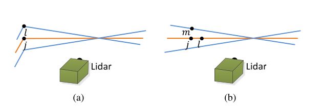
Fig. 7. Finding an edge line as the correspondence for an edge point in ${\tilde{\mathcal{E}}}_{k+1}$ (a), and a planar patch as the correspondence for a planar point in ${\tilde{\mathcal{H}}}_{k+1}$ (b). In both (a) and (b), $j$ is the closest point to the feature point, found in ${\mathcal{P}}_k$. The orange colored lines represent the same scan of $j$, and the blue colored lines are the two consecutive scans. To find the edge line correspondence in (a), we find another point, $l$, on the blue colored lines, and the correspondence is represented as $(j,l)$. To find the planar patch correspondence in (b), we find another two points, $l$ and $m$, on the orange and blue colored lines, respectively. The correspondence is $(j,l,m)$.
图7。（a）表示在${\tilde{\mathcal{E}}}_{k+1}$中如何查找对应的线点，（b）表示在${\tilde{\mathcal{H}}}_{k+1}$中如何查找对应的面点。在（a）和（b）中，$j$是距离特征点最近的点，位于${\mathcal{P}}_k$中。橙色线条表示$j$的同一次扫描，蓝色线条表示两次连续扫描。为了找到（a）中的边线对应关系，我们在蓝色线上找到另一个点，$l$，对应关系表示为$（j，l）$。为了找到（b）中的平面面片对应关系，我们在橙色和蓝色线上分别找到另外两个点，$l$和$m$。对应关系为$（j，l，m）$。

Fig. 7(b) shows the procedure of finding a planar patch as the correspondence of a planar point. Let $i$ be a point in ${\tilde{\mathcal{H}}}_{k+1}$, $i\in {\tilde{\mathcal{H}}}_{k+1}$. The planar patch is represented by three points. Similar to the last paragraph, we find the closest neighbor of $i$ in ${\overline{\mathcal{P}}}_k$, denoted as $j$. Then, we find another two points, $l$ and $m$, as the closest neighbors of $i$, one in the same scan of $j$, and the other in the two consecutive scans to the scan of $j$. This guarantees that the three points are non-collinear. To verify that $j,l$, and $m$ are all planar points, we check again the smoothness of the local surface based on (1).
图7（b）示出了寻找作为平面点对应的平面面片的过程。设$i$为${\tilde{\mathcal{H}}}_{k+1}$中的一个点， $i\in {\tilde{\mathcal{H}}}_{k+1}$。平面面片由三个点表示。与上一段类似，我们在$\overline{\mathcal{P}}k$中找到$i$的最近邻，表示为$j$。然后，我们发现另外两个点，$l$和$m$是$i$的最近邻点，一个在$j$的相同扫描中，另一个在$j$的两个连续扫描中。这保证了三个点不共线。为了验证$j、l$和$m$都是平面点，我们根据（1）再次检查局部曲面的平滑度。

若$j$和$l$也不在同一条线上的话，会存在三个点都在竖直方向上共线的风险

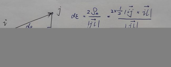
With the correspondences of the feature points found, now we derive expressions to compute the distance from a feature point to its correspondence. We will recover the lidar motion by minimizing the overall distances of the feature points in the next section. We start with edge points. For a point $i\in {\tilde{\mathcal{E}}}_{k+1}$, if $(j,l)$ is the corresponding edge line, $j,l\in {\overline{\mathcal{P}}}_k$, the point to line distance can be computed as
根据找到的特征点的对应关系，现在我们导出表达式来计算从特征点到其对应关系的距离。在下一节中，我们将通过最小化特征点的总距离来恢复激光雷达运动。我们从边缘点开始。对于点$i\in {\tilde{\mathcal{E}}}_{k+1}$，如果$（j，l）$是对应的边线，$j，l\in {\overline{\mathcal{P}}}_k$，则点到线的距离可以计算为

将重新投影的点云表示为${\overline{P}}_k$(k时刻的点云投影到k+1时刻)
使用当前估计的变换将${\mathcal{E}}_{k+1}$和${\mathcal{H}}_{k+1}$重新投影到扫描的开始。${\tilde{\mathbf{X}}}_{(k+1,i)}^L$表示为k+1时刻的点云重新投影到k时刻

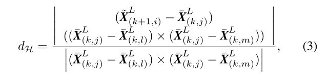
where ${\tilde{\mathbf{X}}}_{(k+1,i)}^L,{\overline{\mathbf{X}}}_{(k,j)}^L$, and ${\overline{\mathbf{X}}}_{(k,l)}^L$ are the coordinates of points $i,j$, and $l$ in $\{L\}$, respectively. Then, for a point $i\in {\tilde{\mathcal{H}}}_{k+1}$, if $(j,l,m)$ is the corresponding planar patch, $j,l,m\in {\overline{\mathcal{P}}}_k$, the point to plane distance is
其中${\tilde{\mathbf{X}}}_{(k+1,i)}^L,{\overline{\mathbf{X}}}_{(k,j)}^L$, 和 ${\overline{\mathbf{X}}}_{(k,l)}^L$ 分别是$L$中点$i，j$和$l$的坐标。然后，对于点$i\in {\tilde{\mathcal{H}}}_{k+1}$，如果$（j，l，m）$是对应的平面面片，$j，l，m\in {\overline{\mathcal{P}}}_k$，则点到平面的距离为

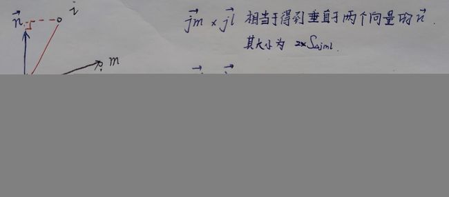
求取点到平面的距离最小相当于让向量ij到向量jn的投影的模长最小

where ${\overline{\mathbf{X}}}_{(k,m)}^L$ is the coordinates of point $m$ in $\{L\}$.
其中 ${\overline{\mathbf{X}}}_{(k,m)}^L$ 是点$m$在$\{L\}$中的坐标

C. Motion Estimation

The lidar motion is modeled with constant angular and linear velocities during a sweep. This allows us to linear interpolate the pose transform within a sweep for the points that are received at different times. Let $t$ be the current time stamp, and recall that $t_{k+1}$ is the starting time of sweep $k+1$. Let ${\mathbf{T}}_{k+1}^L$ be the lidar pose transform between $\left[t_{k+1},t\right]$. $T_{k+1}^L$ contains rigid motion of the lidar in 6-DOF, $T_{k+1}^L=$ ${\left[t_x,t_y,t_z,{\theta }_x,{\theta }_y,{\theta }_z\right]}^T$, where $t_x,t_y$, and $t_z$ are translations along the $x-,y-$, and $z$ - axes of $\{L\}$, respectively, and ${\theta }_x$, ${\theta }_y$, and ${\theta }_z$ are rotation angles, following the right-hand rule. Given a point $i,i\in {\mathcal{P}}_{k+1}$, let $t_i$ be its time stamp, and let ${\mathbf{T}}_{(k+1,i)}^L$ be the pose transform between $\left[t_{k+1},t_i\right].{\mathbf{T}}_{(k+1,i)}^L$ can be computed by linear interpolation of $T_{k+1}^L$,
激光雷达运动在扫描过程中以恒定的角速度和线速度进行建模。这允许我们在扫描中对在不同时间接收到的点进行线性插值计算姿势变换。让$t$作为当前时间戳，并记住$t_{k+1}$是第$k+1$次扫描的开始时间。设${\mathbf{T}}_{k+1}^L$为$\left[T_{k+1}，T\right]$之间的激光雷达姿态变换。$T_{k+1}^L$包含激光雷达在6-DOF中的刚体运动，$T_{k+1}^L=$ ${\left[t_x,t_y,t_z,{\theta }_x,{\theta }_y,{\theta }_z\right]}^T$,其中 $t_x,t_y$, 和 $t_z$分别表示为沿着{L}的x，y和z轴的平移，${\theta }_x$, ${\theta }_y$, and ${\theta }_z$表示为绕轴的旋转角度，遵循右手规则。给定一个点$i，i\in {\mathcal{P}}_{k+1}$，让$t_i$作为它的时间戳，让${\mathbf{T}}_{(k+1,i)}^L$作为$\left[t_{k+1},t_i\right]$之间的姿势变换。${\mathbf{T}}_{(k+1,i)}^L$可以通过$T_{k+1}^L$的线性插值来计算，

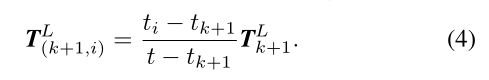
Recall that ${\mathcal{E}}_{k+1}$ and ${\mathcal{H}}_{k+1}$ are the sets of edge points and planar points extracted from ${\mathcal{P}}_{k+1}$, and ${\tilde{\mathcal{E}}}_{k+1}$ and ${\tilde{\mathcal{H}}}_{k+1}$ are the sets of points reprojected to the beginning of the sweep, $t_{k+1}$. To solved the lidar motion, we need to establish a geometric relationship between ${\mathcal{E}}_{k+1}$ and ${\tilde{\mathcal{E}}}_{k+1}$, or ${\mathcal{H}}_{k+1}$ and ${\tilde{\mathcal{H}}}_{k+1}$. Using the transform in (4), we can derive,
回想一下， ${\mathcal{E}}_{k+1}$和 ${\mathcal{H}}_{k+1}$ 是从${\mathcal{P}}_{k+1}$中提取的边点和平面点集，而${\tilde{\mathcal{E}}}_{k+1}$ 和 ${\tilde{\mathcal{H}}}_{k+1}$是重新投影到扫描开始的点集。为了得到激光雷达的运动，我们需要在${\mathcal{E}}_{k+1}$和 ${\tilde{\mathcal{E}}}_{k+1}$，或者${\mathcal{H}}_{k+1}$ 和 ${\tilde{\mathcal{H}}}_{k+1}$之间建立几何关系。使用（4）中的变换，我们可以得出，

where ${\mathbf{X}}_{(k+1,i)}^L$ is the coordinates of a point $i$ in ${\mathcal{E}}_{k+1}$ or ${\mathcal{H}}_{k+1},{\tilde{\mathbf{X}}}_{(k+1,i)}^L$ is the corresponding point in ${\tilde{\mathcal{E}}}_{k+1}$ or ${\tilde{\mathcal{H}}}_{k+1}$, ${\mathbf{T}}_{(k+1,i)}^L(a:b)$ is the $a$-th to $b$-th entries of ${\mathbf{T}}_{(k+1,i)}^L$, and $\mathbf{R}$ is a rotation matrix defined by the Rodrigues formula [25],
其中${\mathbf{X}}_{(k+1,i)}^L$是点 $i$在 ${\mathcal{E}}_{k+1}$ 或 ${\mathcal{H}}_{k+1}$的坐标，${\tilde{\mathbf{X}}}_{(k+1,i)}^L$是点i在${\tilde{\mathcal{E}}}_{k+1}$ or ${\tilde{\mathcal{H}}}_{k+1}$中的对应点。${\mathbf{T}}_{(k+1,i)}^L(a:b)$是 ${\mathbf{T}}_{(k+1,i)}^L$的第a到第b个条目，而 $\mathbf{R}$是由罗德里格斯公式定义的旋转矩阵[25]

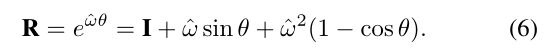
In the above equation, $\theta$ is the magnitude of the rotation,
在上面的等式中，$\theta$是旋转的幅度，

$\omega$ is a unit vector representing the rotation direction,
$\omega$是表示旋转方向的单位向量，

and $\hat{\omega }$ is the skew symmetric matrix of $\omega$ [25].
$\hat{\omega }$是$\omega$[25]的斜对称矩阵。

Recall that $(2)$ and $(3)$ compute the distances between points in ${\tilde{\mathcal{E}}}_{k+1}$ and ${\mathcal{H}}_{k+1}$ and their correspondences. Combining $(2)$ and (4)-(8), we can derive a geometric relationship between an edge point in ${\mathcal{E}}_{k+1}$ and the corresponding edge line,
回想一下，$（2）$和$（3）$计算${\tilde{E}}_{k+1}$和${\mathcal{H}}_{k+1}$中点之间的距离及其对应关系。结合$（2）$和（4）-（8），我们可以导出$\mathcal{E}k+1$中的边点与相应边线之间的几何关系，

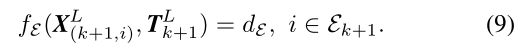
Similarly, combining (3) and (4)-(8), we can establish another geometric relationship between a planar point in ${\mathcal{H}}_{k+1}$ and the corresponding planar patch,

类似地，结合（3）和（4）-（8），我们可以在${\mathcal{H}}_{k+1}$中的平面点和相应的planar patch之间建立另一个几何关系，
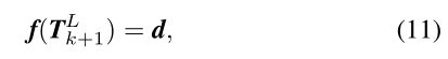
Finally, we solve the lidar motion with the LevenbergMarquardt method [26]. Stacking $(9)$ and (10) for each feature point in ${\mathcal{E}}_{k+1}$ and ${\mathcal{H}}_{k+1}$, we obtain a nonlinear function,
最后，我们使用LevenbergMarquardt方法求解激光雷达运动[26]。对${\mathcal{E}}_{k+1}$和 ${\mathcal{H}}_{k+1}$中的每个特征点叠加$（9）$和 (10)，我们得到一个非线性函数，

求解变换矩阵T从而让两个d(残差:点到线的距离和点到面的距离)最小

where each row of $f$ corresponds to a feature point, and $d$ contains the corresponding distances. We compute the Jacobian matrix of $\mathbf{f}$ with respect to ${\mathbf{T}}_{k+1}^L$, denoted as $\mathbf{J}$, where $\mathbf{J}=\partial f/\partial {\mathbf{T}}_{k+1}^L.$ Then, 11 can be solved through nonlinear iterations by minimizing $\mathbf{d}$ toward zero,
其中，$f$的每一行对应一个特征点，$d$包含相应的距离。我们计算$\mathbf{f}$关于${\mathbf{T}}_{k+1}^L$的雅可比矩阵，表示为$\mathbf{J}$，其中$\mathbf{J}=\partial f/\partial {\mathbf{T}}_{k+1}^L$ 。 然后，（11）可以通过非线性迭代求解，将$\mathbf{d}$最小化为零，

$\lambda$ is a factor determined by the Levenberg-Marquardt method.
$\lambda$是由Levenberg-Marquardt方法确定的系数。

D. Lidar Odometry Algorithm

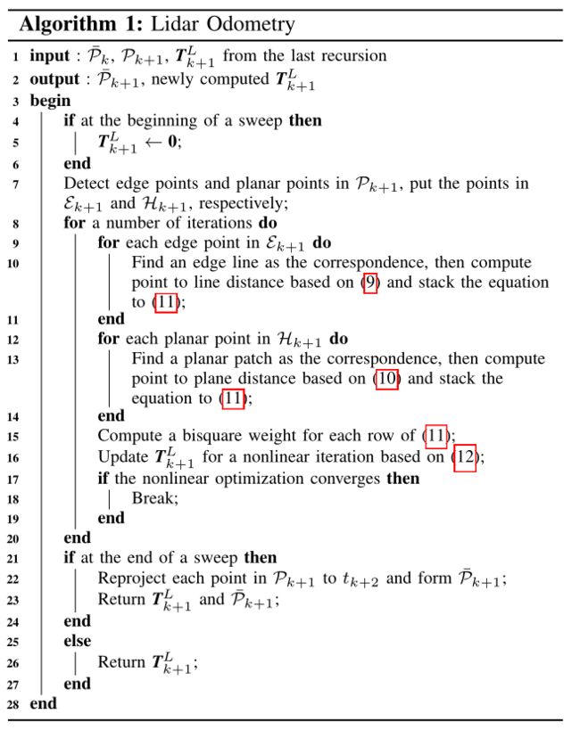
The lidar odometry algorithm is shown in Algorithm 1 . The algorithm takes as inputs the point cloud from the last sweep, ${\overline{\mathcal{P}}}_k$, the growing point cloud of the current sweep, ${\mathcal{P}}_{k+1}$, and the pose transform from the last recursion, $T_{k+1}^L.$ If a new sweep is started, $T_{k+1}^L$ is set to zero (line 4-6). Then, the algorithm extracts feature points from ${\mathcal{P}}_{k+1}$ to construct ${\mathcal{E}}_{k+1}$ and ${\mathcal{H}}_{k+1}$ in line 7. For each feature point, we find its correspondence in ${\overline{\mathcal{P}}}_k$ (line 9-19). The motion estimation is adapted to a robust fitting [27]. In line 15, the algorithm assigns a bisquare weight for each feature point. The feature points that have larger distances to their correspondences are assigned with smaller weights, and the feature points with distances larger than a threshold are considered as outliers and assigned with zero weights. Then, in line 16, the pose transform is updated for one iteration. The nonlinear optimization terminates if convergence is found, or the maximum iteration number is met. If the algorithm reaches the end of a sweep, ${\mathcal{P}}_{k+1}$ is reprojected to time stamp $t_{k+2}$ using the estimated motion during the sweep. Otherwise, only the transform $T_{k+1}^L$ is returned for the next round of recursion.
激光雷达里程计算法如Algorithm 1 所示。该算法将最后一次扫描的点云$\overline{\mathcal{P}}k$、当前扫描的增长点云${\mathcal{P}}_{k+1}$和最后一次递归的姿势变换$T_{k+1}^{L} $ 作为输入。如果开始新的扫描，$T_{k+1}^L$被设置为零（第4-6行）。然后，该算法从${\mathcal{P}}_{K+1}$中提取特征点，在第7行构造${\mathcal{E}}_{k+1}$和${\mathcal{H}}_{k+1}$ 。对于每个特征点，我们在${\overline{\mathcal{P}}}_k$（第9-19行）中找到其对应关系。运动估计适用于鲁棒拟合（robust fitting）[27]。在第15行中，算法为每个特征点分配一个双平方权重。对与其对应点距离较大的特征点分配较小的权重，对距离大于阈值的特征点视为异常值并分配零权重。然后，在第16行中，姿势变换更新一次迭代。如果发现收敛或满足最大迭代次数，则非线性优化终止。如果算法到达扫描结束时，${\mathcal{P}}_{k+1}$将使用扫描期间的估计运动重新投影到时间戳$t_{k+2}$。否则，下一轮递归只返回转换$T_{k+1}^L$。

VI. LIDAR MAPPING

The mapping algorithm runs at a lower frequency then the odometry algorithm, and is called only once per sweep. At the end of sweep $k+1$, the lidar odometry generates a undistorted point cloud, ${\overline{\mathcal{P}}}_{k+1}$, and simultaneously a pose transform, $T_{k+1}^L$, containing the lidar motion during the sweep, between $\left[t_{k+1},t_{k+2}\right]$. The mapping algorithm matches and registers ${\overline{\mathcal{P}}}_{k+1}$ in the world coordinates, $\{W\}$, illustrated in Fig. 8. To explain the procedure, let us define ${\mathcal{Q}}_k$ as the point cloud on the map, accumulated until sweep $k$, and let ${\mathbf{T}}_k^W$ be the pose of the lidar on the map at the end of sweep $k$, $t_{k+1}$. With the outputs from the lidar odometry, the mapping algorithm extents $T_k^W$ for one sweep from $t_{k+1}$ to $t_{k+2}$, to obtain $T_{k+1}^W$, and projects ${\overline{\mathcal{P}}}_{k+1}$ into the world coordinates, $\{W\}$, denoted as ${\overline{\mathcal{Q}}}_{k+1}.$ Next, the algorithm matches ${\overline{\mathcal{Q}}}_{k+1}$ with ${\mathcal{Q}}_k$ by optimizing the lidar pose $T_{k+1}^W$.
mapping算法的运行频率低于里程计算法，每次扫描只调用一次。在第$k+1$次扫描结束时，激光雷达里程计生成一个去畸变的点云，${\overline{\mathcal{P}}}_{K+1}$，同时生成一个$\left[t_{k+1},t_{k+2}\right]$之间的姿势变换，$T_{k+1}^L$，包含扫描期间的激光雷达运动 。mapping算法将${\overline{\mathcal{P}}}_{K+1}$在世界坐标$\{W\}$中匹配并对齐，如图8所示。为了解释这个过程，我们将${\mathcal{Q}}_K$定义为地图上的点云，累积到第$k$次扫描，并将${\mathbf{T}}_K^W$定义为 第$k$次扫描，$T_{k+1}$结束时地图上激光雷达的姿态。利用激光雷达里程计的输出，mapping算法将$T_k^W$从$T_{k+1}$扩展到$T_{k+2}$，以获得$T_{k+1}^W$，并将${\overline{\mathcal{P}}}_{k+1}$投影到世界坐标$W$，表示为${\overline{\mathcal{Q}}}_{k+1}.$接下来，该算法通过优化lidar姿态$T_{k+1}$将${\overline{\mathcal{Q}}}_{k+1}$与${\mathcal{Q}}_k$进行匹配。

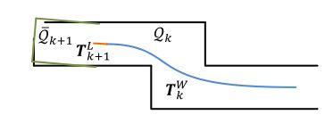
Fig. 8. Illustration of mapping process. The blue colored curve represents the lidar pose on the map, $T_k^W$, generated by the mapping algorithm at sweep $k$. The orange color curve indicates the lidar motion during sweep $k+1,T_{k+1}^L$, computed by the odometry algorithm. With ${\mathbf{T}}_k^W$ and ${\mathbf{T}}_{k+1}^L$, the undistorted point cloud published by the odometry algorithm is projected onto the map, denoted as ${\mathcal{Q}}_{k+1}$ (the green colored line segments), and matched with the existing cloud on the map, ${\mathcal{Q}}_k$ (the black colored line segments).
图8.mapping过程的图示。蓝色曲线表示地图上的激光雷达姿态，$T_k^W$，由第$k$次扫描的mapping算法生成。橙色曲线表示由里程计算法计算的第$k+1$次扫描,$T_{k+1}^L$期间的激光雷达运动。使用${\mathbf{T}}_k^W$和${\mathbf{T}}_{k+1}^L$将里程计算法发布的去畸变后的点云投影到地图上，表示为${\mathcal{Q}}_{k+1}$（绿色线段），并与地图上的现有点云${\mathcal{Q}}_K$（黑色线段）匹配。

${\mathcal{Q}}_{k+1}$为最新帧投影到开始时的点云

The feature points are extracted in the same way as in Section V -A, but 10 times of feature points are used. To find correspondences for the feature points, we store the point cloud on the map,$Q_k$, in 10m cubic areas. The points in the cubes that intersect with ${\overline{Q}}_{k+1}$ are extracted and stored in a 3D KD-tree [24]. We find the points in $Q_k$ within a certain region around the feature points. Let $S^{\prime }$ be a set of surrounding points. For an edge point, we only keep points on edge lines in $S^{\prime }$, and for a planar point, we only keep points on planar patches. Then, we compute the covariance matrix of $S^{\prime }$, denoted as $M$, and the eigenvalues and eigenvectors of $M$, denoted as $V$ and $E$, respectively. If $S^{\prime }$ is distributed on an edge line, $V$contains one eigenvalue significantly larger than the other two, and the eigenvector in $E$ associated with the largest eigenvalue represents the orientation of the edge line. On the other hand, if $S^{\prime }$ is distributed on a planar patch,$V$ contains two large eigenvalues with the third one significantly smaller, and the eigenvector in $E$ associated with the smallest eigenvalue denotes the orientation of the planar patch. The position of the edge line or the planar patch is determined by passing through the geometric center of $S^{\prime }$.
特征点的提取方法与第V-A节相同（但是是在地图中找匹配点），但使用了10倍的特征点。为了找到特征点的对应关系，我们将点云存储在地图$Q_k$上，以10立方米的大小存储。立方体中与${\overline{Q}}_{k+1}$相交的点被提取并存储在3D KD树中[24]。我们在$Q_k$中寻找特征点周围的一定区域内的点。设$S^{\prime }$为一组周围点。对于边点，我们只在$S^{\prime }$中保留边线上的点，对于平面点，我们只保留在planar patches上的点。然后，我们计算$S^{\prime }$的协方差矩阵，表示为$M$，$M$的特征值和特征向量，表示为$V$和$E$。如果$S^{\prime }$分布在边缘线上，$V$包含一个显著大于其他两个的特征值，$E$中与最大特征值相关的特征向量表示边缘线的方向。另一方面，如果$S^{\prime }$分布在一个 planar patch上，$V$包含两个较大的特征值，第三个特征值明显较小，$E$中与最小特征值相关的特征向量表示平面patch的方向（法向量）。边线或 planar patch的位置通过$S^{\prime }$的几何中心确定。

To compute the distance from a feature point to its correspondence, we select two points on an edge line, and three points on a planar patch. This allows the distances to be computed using the same formulations as (2) and (3). Then, an equation is derived for each feature point as (9) or (10), but different in that all points in ${\overline{Q}}_{k+1}$ share the same time stamp,$t_{k+2}$. The nonlinear optimization is solved again by a robust fitting [27] through the Levenberg-Marquardt method [26], and ${\overline{Q}}_{k+1}$ is registered on the map. To evenly distribute the points, the map cloud is downsized by a voxel grid filter [28] with the voxel size of 5cm cubes
为了计算从特征点到其对应点的距离，我们在边线上选择两个点，在planar patch上选择三个点。这允许使用与（2）和（3）相同的公式计算距离。然后，基于（9）或（10）将每个特征点的方程导出，但不同之处在于${\overline{Q}}_{k+1}$ 中的所有点都具有相同的时间戳$t_{k+2}$。使用Levenberg-Marquardt方法[26]通过robust拟合[27]可以再次解决非线性优化问题，并且${\overline{Q}}_{k+1}$在地图上registered。为了均匀分布点，地图点云通过体素网格过滤器[28]缩小为体素大小为5cm的立方体（下采样，每个立方体中保留一个点）

Integration of the pose transforms is illustrated in Fig. 9. The blue colored region represents the pose output from the lidar mapping,$T_k^W$, generated once per sweep. The orange colored region represents the transform output from the lidar odometry, $T_{k+1}^L$, at a frequency round 10Hz. The lidar pose with respect to the map is the combination of the two transforms, at the same frequency as the lidar odometry.
姿势变换的集成(intergration)如图9所示。蓝色区域表示激光雷达mapping输出的姿势，$T_k^W$，每次扫描生成一次。橙色区域表示激光雷达里程计输出的变换（transform），$T_{k+1}^L$，频率约为10Hz。相对于地图的激光雷达姿态是两个变换的组合，频率与激光雷达里程计相同。

Fig. 9. Integration of pose transforms. The blue colored region illustrates the lidar pose from the mapping algorithm,$T_k^W$, generated once per sweep. The orange colored region is the lidar motion within the current sweep,$T_{k+1}^L$, computed by the odometry algorithm. The motion estimation of the lidar is the combination of the two transforms, at the same frequency as $T_{k+1}^L$
图9。姿势变换的集成。蓝色区域显示了mapping算法中的激光雷达姿态，$T_k^W$，每次扫描生成一次。橙色区域是当前扫描范围内的激光雷达运动，$T_{k+1}^L$，由里程计算法计算。激光雷达的运动估计是两种变换的组合，频率与$T_{k+1}^L$相同

VII. EXPERIMENTS

VIII. CONCLUSION ANDFUTUREWORK

Motion estimation and mapping using point cloud from a rotating laser scanner can be difficult because the problem involves recovery of motion and correction of motion distortion in the lidar cloud. The proposed method divides and solves the problem by two algorithms running in parallel: the lidar odometry conduces coarse processing to estimate velocity at a higher frequency, while the lidar mapping performs fine processing to create maps at a lower frequency. Cooperation of the two algorithms allows accurate motion estimation and mapping in real-time. Further, the method can take advantage of the lidar scan pattern and point cloud distribution. Feature matching is made to ensure fast computation in the odometry algorithm, and to enforce accuracy in the mapping algorithm. The method has been tested both indoor and outdoor as well as on the KITTI odometry benchmark.
使用旋转激光扫描仪的点云进行运动估计和建图可能很困难，因为该问题涉及到恢复激光雷达云中的运动和校正运动失真。所提出的方法通过两种并行运行的算法来解决该问题：激光雷达里程计（算法）进行粗处理以估计较高频率的速度，而激光雷达mapping（算法）进行精细处理以创建较低频率的地图。这两种算法的合作允许实时精确的运动估计和建图。此外，该方法可以利用激光雷达扫描模式和点云分布的优势。特征匹配是为了保证里程计算法的快速计算，并提高映射算法的准确性。该方法已在室内外以及KITTI里程计基准上进行了测试。

Since the current method does not recognize loop closure, our future work involves developing a method to fix motion estimation drift by closing the loop. Also, we will integrate the output of our method with an IMU in a Kalman filter to further reduce the motion estimation drift.
由于目前的方法不识别loop closure，我们未来的工作涉及开发一种通过loop closure来修复运动估计漂移的方法。此外，我们还将我们的方法的输出与卡尔曼滤波器中的IMU集成，以进一步减小运动估计漂移。