TSNE实现降维及可视化
目录
- 前言
- 降维
- 可视化
- 举例:
前言
- 最近在看迁移学习需要观察迁移效果,需要把特征可视化来查看分布情况,所以需要用到降维可视化这个工具,所以在这里记录一下。
- 方法挺简单的,阅读本文大概5分钟。
降维
- 使用TSNE进行降维操作,该函数的输入是flatten之后的特征,即[batch,维度]。
- 接口参数解释:
sklearn.manifold.TSNE(n_components=2, perplexity=30.0, early_exaggeration=12.0, learning_rate=200.0, n_iter=1000, n_iter_without_progress=300, min_grad_norm=1e-07, metric=’euclidean’, init=’random’, verbose=0, random_state=None, method=’barnes_hut’, angle=0.5)
参数:
n_components:int,可选(默认值:2)嵌入式空间的维度。
perplexity:浮点型,可选(默认:30)较大的数据集通常需要更大的perplexity。考虑选择一个介于5和50之间的值。由于t-SNE对这个参数非常不敏感,所以选择并不是非常重要。
early_exaggeration:float,可选(默认值:4.0)这个参数的选择不是非常重要。
learning_rate:float,可选(默认值:1000)学习率可以是一个关键参数。它应该在100到1000之间。如果在初始优化期间成本函数增加,则早期夸大因子或学习率可能太高。如果成本函数陷入局部最小的最小值,则学习速率有时会有所帮助。
n_iter:int,可选(默认值:1000)优化的最大迭代次数。至少应该200。
n_iter_without_progress:int,可选(默认值:300,必须是50倍数)在我们中止优化之前,没有进展的最大迭代次数。
0.17新版功能:参数n_iter_without_progress控制停止条件。
min_grad_norm:float,可选(默认值:1E-7)如果梯度范数低于此阈值,则优化将被中止。
metric:字符串或可迭代的,可选,计算特征数组中实例之间的距离时使用的度量。如果度量标准是字符串,则它必须是scipy.spatial.distance.pdist为其度量标准参数所允许的选项之一,或者是成对列出的度量标准.PAIRWISE_DISTANCE_FUNCTIONS。如果度量是“预先计算的”,则X被假定为距离矩阵。或者,如果度量标准是可调用函数,则会在每对实例(行)上调用它,并记录结果值。可调用应该从X中获取两个数组作为输入,并返回一个表示它们之间距离的值。默认值是“euclidean”,它被解释为欧氏距离的平方。
init:字符串,可选(默认值:“random”)嵌入的初始化。可能的选项是“随机”和“pca”。 PCA初始化不能用于预先计算的距离,并且通常比随机初始化更全局稳定。
random_state:int或RandomState实例或None(默认)
伪随机数发生器种子控制。如果没有,请使用numpy.random单例。请注意,不同的初始化可能会导致成本函数的不同局部最小值。
method:字符串(默认:‘barnes_hut’)
默认情况下,梯度计算算法使用在O(NlogN)时间内运行的Barnes-Hut近似值。 method ='exact’将运行在O(N ^ 2)时间内较慢但精确的算法上。当最近邻的误差需要好于3%时,应该使用精确的算法。但是,确切的方法无法扩展到数百万个示例。0.17新版功能:通过Barnes-Hut近似优化方法。
angle:float(默认值:0.5)
仅当method ='barnes_hut’时才使用这是Barnes-Hut T-SNE的速度和准确性之间的折衷。 ‘angle’是从一个点测量的远端节点的角度大小(在[3]中称为theta)。如果此大小低于’角度’,则将其用作其中包含的所有点的汇总节点。该方法对0.2-0.8范围内该参数的变化不太敏感。小于0.2的角度会迅速增加计算时间和角度,因此0.8会快速增加误差。
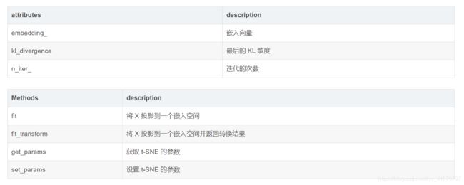
- 这部分不用了解太多,知道几个主要的参数如n_components、n_iter、init等以及主要的方法fit_transform就好了。
可视化
- 这一部分自己构造函数。
- 二维可视化:
def plot_embedding_2d(X, y, d, title=None):
    """Plot an embedding X with the class label y colored by the domain d."""
    x_min, x_max = np.min(X, 0), np.max(X, 0)
    X = (X - x_min) / (x_max - x_min)

    # Plot colors numbers
    plt.figure(figsize=(10,10))
    ax = plt.subplot(111)
    for i in range(X.shape[0]):
        # plot colored number
        plt.text(X[i, 0], X[i, 1], str(y[i]),
                 color=plt.cm.bwr(d[i] / 1.),
                 fontdict={'weight': 'bold', 'size': 9})

    plt.xticks([]), plt.yticks([])
    if title is not None:
        plt.title(title)
上面的函数大家自己可以修改,就画个图而已,降维后的数据都给你了。因为我是迁移学习,所以添加了每条数据的域类别d。另外,大家根据自己的分类类别设置plt.cm.Set或者bwr。
- 三维可视化:
def plot_embedding_3d(X, title=None):
    #坐标缩放到[0,1]区间
    x_min, x_max = np.min(X,axis=0), np.max(X,axis=0)
    X = (X - x_min) / (x_max - x_min)
    #降维后的坐标为(X[i, 0], X[i, 1],X[i,2]),在该位置画出对应的digits
    fig = plt.figure()
    ax = fig.add_subplot(1, 1, 1, projection='3d')
    for i in range(X.shape[0]):
        ax.text(X[i, 0], X[i, 1], X[i,2],str(digits.target[i]),
                 color=plt.cm.Set1(y[i] / 10.),
                 fontdict={'weight': 'bold', 'size': 9})
    if title is not None:
        plt.title(title)
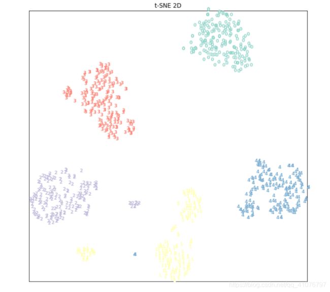
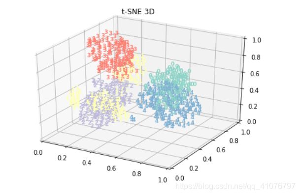
举例:
- 代码:
from sklearn import datasets
from sklearn.manifold import TSNE
import numpy as np
import matplotlib.pyplot as plt
digits = datasets.load_digits(n_class=5)
X = digits.data
y = digits.target
print(X.shape) # 901,64

def plot_embedding_2d(X, y, title=None):
    """Plot an embedding X with the class label y colored by the domain d."""
    x_min, x_max = np.min(X, 0), np.max(X, 0)
    X = (X - x_min) / (x_max - x_min)

    # Plot colors numbers
    plt.figure(figsize=(10,10))
    ax = plt.subplot(111)
    for i in range(X.shape[0]):
        # plot colored number
        plt.text(X[i, 0], X[i, 1], str(y[i]),
                 color=plt.cm.Set3(y[i] / 10.),
                 fontdict={'weight': 'bold', 'size': 9})

    plt.xticks([]), plt.yticks([])
    if title is not None:
        plt.title(title)
    plt.show()

def plot_embedding_3d(X,y, title=None):
    #坐标缩放到[0,1]区间
    x_min, x_max = np.min(X,axis=0), np.max(X,axis=0)
    X = (X - x_min) / (x_max - x_min)
    #降维后的坐标为(X[i, 0], X[i, 1],X[i,2]),在该位置画出对应的digits
    fig = plt.figure()
    #ax = fig.add_subplot(1, 1, 1, projection='3d')
    ax = Axes3D(fig)
    for i in range(X.shape[0]):
        ax.text(X[i, 0], X[i, 1], X[i,2],str(digits.target[i]),
                 color=plt.cm.Set3(y[i] / 10.),
                 fontdict={'weight': 'bold', 'size': 9})
    if title is not None:
        plt.title(title)
    plt.show()

print("Computing t-SNE embedding")
tsne2d = TSNE(n_components=2, init='pca', random_state=0)
tsne3d = TSNE(n_components=3, init='pca', random_state=0)

X_tsne_2d = tsne2d.fit_transform(X)
X_tsne_3d = tsne3d.fit_transform(X)
plot_embedding_2d(X_tsne_2d[:,0:2],y,"t-SNE 2D")
plot_embedding_3d(X_tsne_3d[:,0:3],y,"t-SNE 3D")
效果: