【论文阅读】Scene Text Image Super-Resolution in the Wild

摘要

TextZoom：真实的场景文本SR数据集，包含了成对的真实的低分辨率和高分辨率的图像，是由不同焦距的相机在野外拍摄的。它比合成数据更真实，也更具挑战性。
文本超分辨率网络TSRN：（1）提出了一个序列残差块来提取文本图像的序列信息。（2）提出一种边界感知损失，旨在锐化字符边界。（3）提出了一个中心对齐模块来缓解文本缩放中的错位问题。
本文成果：在TextZoom上的大量实验表明，与合成SR数据相比，TSRN大大提高了CRNN的13%以上，提高了CRNN和MORAN的近9.0%。TSRN在提高TextZoom中LR图像的识别精度方面明显优于7种最先进的SR方法。

引言

介绍超分辨率以及文本图像超分辨率的背景和重要性
在识别图片中的文字前引入SR方法作为一种预处理程序会对后续识别帮助很大
本文提出的TextZoom是第一个关注真实文本SR的数据集，有以下三个优势：（1）有很好的注释。提供了文本图像的方向、文本内容和原始焦距。（2）包含了来自不同自然场景的丰富文本，包括街景、图书馆、商店、汽车内饰等。（3）数据集按难度分为三个子集。
提出了一种面向文本的端到端方法：场景文本SR与传统SR不同之处在于，传统的SR只需要注重纹理细节即可。场景文本SR还包含了文本信息，前后的字符之间也有关联，人类可以不用完全看清每个字符也可以识别出这个文本。因此，首先，本文提出了一个序列残差块来建模文本行中的循环信息，这使我们能够在前后字符中建立一个相关性。其次，本文提出了一种边界感知损失称为梯度轮廓损失来重建字符的尖锐边界，这样有助于更好地区分字符和背景，并产生一个更明确的形状。第三，由于相机的不准确，成对图像可能会错位。本文提出了一个中心对齐模块来使相应的像素更对齐。
评估识别精度：（1）对LR文本图像进行超分辨率；（2）使用训练过的文本识别器，如aster、MORAN和CRNN。
本文贡献：1.本文引入了第一个真实的成对场景文本SR数据集文本变焦与不同的焦距。分别用三个子集来注释和分配数据集：易、中和难。 2.通过对比分析合成LR和LR图像训练的模型，证明了该数据集TextZoom的优越性。并从不同的方面证明了场景文本SR的必要性。 3.本文提出了一种新的具有三个新模块的文本超分辨率网络。通过在TextZoom上进行的训练和测试，它明显超过了7种具有代表性的SR方法。

相关工作

超分辨率
文本识别
场景文本超分辨率
但是这些工作的LR图像都是由HR下采样生成的，推广到真实LR图像时还有问题

TextZoom数据集

TextZoom数据集来自于RealSR和SRRAW。这两个新提出的数据集是由数码相机捕获的成对的LR-HR图像组成的。
RealSR包含真实图像、2倍的LR图像、3倍的LR图像、4倍的LR图像。在105mm焦距图像上标注了单词的边界框。
SRRAW拍摄了7种不同焦距的图像，短焦距的图像作为LR图像，长焦距的图像作为相应的真实图像。在240mm焦距图像上标注了单词的边界框
用每一组的最大焦距来标记图像，并从其余的文本框中按照相同的矩形裁剪文本框，因此会产生错位的现象。遇到垂直的图像需要将其转为水平方向的。还有一些曲线文本图像。对于每一对LR-HR图像，也提供了区分大小写的字符串（包括标点符号）、边界框的类型和原始焦距的注释。
选择所有高度从16像素到32像素的图像作为我们的地面真实图像，并向上采样到128×32（宽度×高度），相应的2倍LR图像大小为64×16（宽度×高度）。对于这项任务，由于文本识别的特殊性，只从带注释的文本图像中生成这个2倍LR-HR对数据集。标注的图像的其他尺度的因素可以用于不同的目的。
数据集划分：从RealSR获取的LR图像分为容易。将SR-RAW的LR图像和大于50mm的焦距视为中等。其余的视为难。
本任务主要目的是提高易、中、难子集的识别精度。
峰值信噪比(PSNR)和结构相似性指数(SSIM)：

我们的中和难子集的PSNR不是很好，因为PSNR是像素对像素计算的，而SSIM是用11×11滑动核计算的。中央对齐模块会引入轻微的像素位移，因此PSNR比其他SR方法略低。通常，PSNR和SSIM不能代表图像的视觉质量，在这个任务中，它与准确性相比也不那么重要。
数据集统计信息：

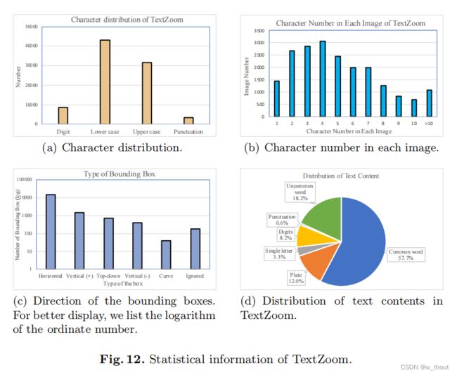
(a)我们的数据集包含丰富的字符和数字，包括一些标点符号。(b)大部分单词的长度范围为1-8个字符。( c)在原始图像中有很多随机放置的方框和书籍，所以我们计算我们标注的边界框的方向类型。“水平”是指文本图像是水平放置的，易于阅读。“垂直（+）”表示文本图像是垂直的，它应该沿顺时针方向旋转90度，而“垂直（-）”表示沿逆时针方向旋转90度。“自上向下”表示文本图像应该旋转180度以获得最佳识别效果。“曲线”表示文本图像为曲线。“忽略”的意思是文本是非法的（不是数字、英文字母或标点符号）。(d)通过ICDAR2015中使用的有9万个通用词汇的通用词汇，我们估计57.5%的文本内容是通用英语单词。车牌包括汽车牌照、车门牌照或路牌。它们是数字、标点符号和字母的组合。这种文字占了12%，因为在原始图片中有很多街景。在所有的文本中占18.2%。这类文本主要是罕见的词、短语或复合词。其他没有意义的字符串，如标点符号、单个字母和数字占了其余的部分。

方法

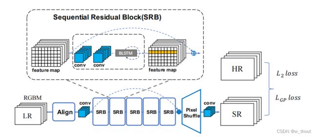
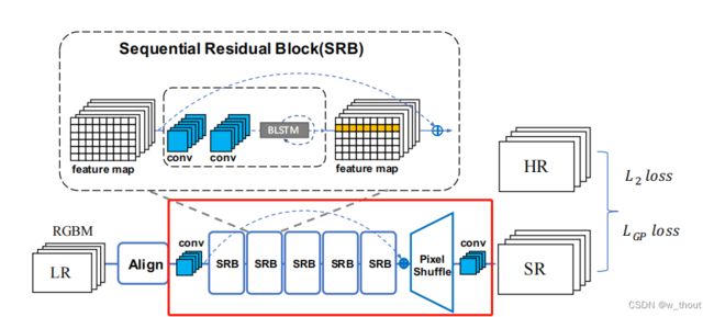
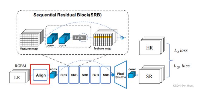
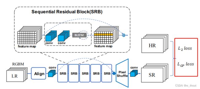
将二进制掩码（通过计算图像的平均灰度来生成的）与RGB通道连接起来作为RGBM 4通道输入。输入由中央对齐模块接收，然后输入到pipeline中。输出的是超分辨率的RGB图像。输出由L2损失监督。输出的RGB通道由LGP损失监督。

pipeline

以SRResNet为基线，在SRResNet的结构上做了两个变化：1)在前面添加了一个中央对齐模块。2)用提议的顺序残差块(SRBs)替换了原来的基本块。在训练过程中，首先，通过中央对准模块对输入进行修正。然后利用CNN层从校正后的图像中提取浅层特征。叠加5个SRB，提取更深层次的顺序依赖特征，并按照ResNet进行快捷连接。最终通过上采样块和CNN生成SR图像。还设计了一个梯度先验损失(LGP)，旨在增强字符的形状边界。网络的输出由MSELoss(L2)和提出的LGP监督。

SRB

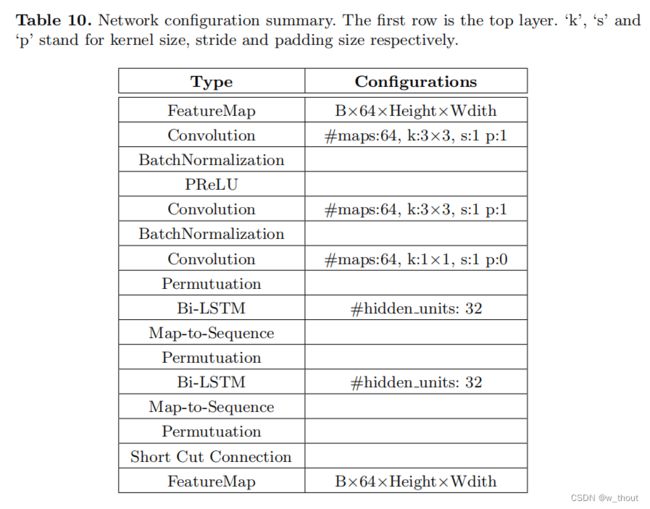
传统的SISR只关心纹理重建，而文本图像具有较强的顺序特征。通过添加双向LSTM(BLSTM)机制对残差块进行了修改。在水平线上建立了序列连接主义，并将该特征融合到更深的通道中。因为构建的网络递归体系结构只是用于低级重构，因此只采用了构建文本行序列依赖的思想。首先，通过CNN提取特征。然后排列和调整特征映射的大小，因为水平的文本行可以被编码成序列。然后，BLSTM可以传播误差差分，将特征映射转化为特征序列，并将其反馈给卷积层。为了使倾斜文本图像的序列依赖性具有鲁棒性，从水平和垂直两个方向引入了BLSTM。BLSTM将水平和垂直卷积特征作为顺序输入，并在隐层中反复地更新其内部状态。

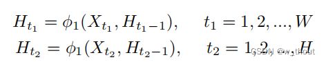
Ht表示隐含层，Xt表示输入特征，t1，t2分别表示从水平和垂直方向的循环连接。

中央对齐模块

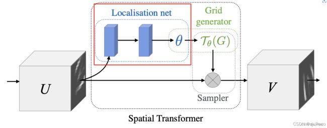
错位使像素到像素的损失，如L1和L2产生显著的伪影和双阴影。因此，引入了STN（Spatial Transformer Network）作为我们的中心对齐模块。STN是一种可以对图像进行整流和端端学习的空间变换网络。为了灵活地修正空间变化，我们采用TPS变换作为变换操作。一旦LR图像中的文本区域与中心相邻对齐，像素级的损失将会产生更好的性能，伪影也可以得到缓解。
中心对齐模块是基于空间转换网络的。该网络预测了一组控制点，然后通过 Thin-Plate-Spline(TPS)变换对图像进行校正。我们的中央对准模块主要使用水平或垂直移动。使用TPS转换来让转换更灵活，可以适应不同的背景区域变换比例。
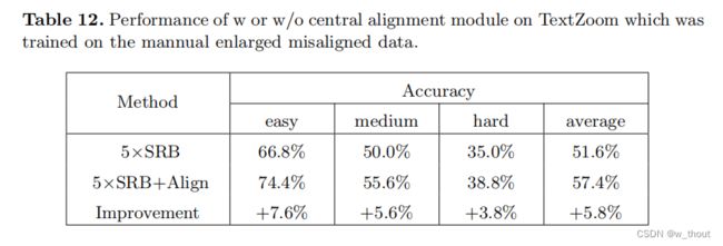
在错位图像对较多的数据集上中央对齐模块可以提高更多的精度。是一个方便的可拔插模块，可以提高SR的性能。

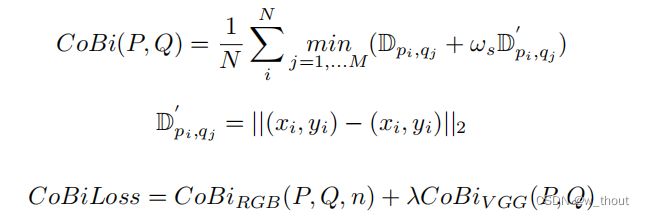
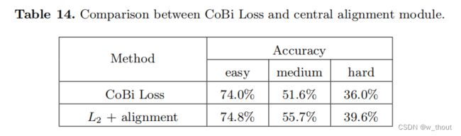
CoBi损失：基于上下文损失的最近邻搜索，并考虑加权空间感知的局部上下文相似性，以此来解决错位问题。CoBi损失使用了预先训练过的VGG-19特征，并选择了几个conv层作为深度特征。由于预先训练的模型是在分类数据集上训练的，所以在这个任务中不太实用。

梯度剖面损失

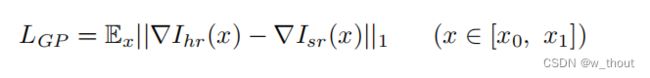
梯度轮廓先验(GPP)，可以在SISR任务中生成更清晰的边缘。梯度场是像素的RGB值的空间梯度。以HR图像的梯度场作为真实值。打磨字符边缘（使其更锐利）可以使字符更明确。GP损失定义如下：

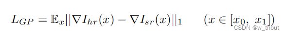
∇Ihr(x)表示HR图像的梯度场，∇Isr(x)表示SR图像的梯度场。

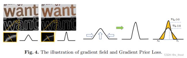
LGP具有两个优点：（1）梯度场生动地显示了文本图像的特征：文本和背景。（2）LR图像的梯度场曲线总是较宽，而HR图像的曲线则较薄。通过数学计算，可以很容易地生成梯度场的曲线。

实验

数据集

TextZoom，为了避免下样本退化，所有的LR图像都被上采样到64×16，而HR图像则被上采样到128×32。

实现细节

将L2损失的权衡权重设为1，LGP设为1e−4。我们使用动量项为0.9的Adam优化器。

文本识别是否需要SR吗？

为了证明文本图像具有超分辨率的必要性，比较了4种方法的识别精度：
1）已发布的方法Released：使用按习惯大小训练的aster模型进行识别（高度不少于32像素，官方发布的模型）。
2）重新实现的方法ReIm：通过在低分辨率图像上训练的模型进行识别(在本工作中，在Syn90K和SynthText上重新实现了aster模型，大小为64×16，除了输入大小外，所有的训练细节都与原始论文相同）
3）微调的方法Fine-tune：微调发布的aster模型
4）本文方法Ours：根据大小选择低分辨率的图像，然后使用本文提出的TSRN来生成SR图像，然后用aster官方发布的模型来识别它们。
从7个常见场景文本测试集IC13、IC15、CUTE、IC03、SVT、SVTP、CUTIT和IIIT5K中选择所有小于64×16的图像，共得到436幅图像。将这个测试集称为CommonLR。在数据集TextZoom和CommonLR上比较了这4种方法。

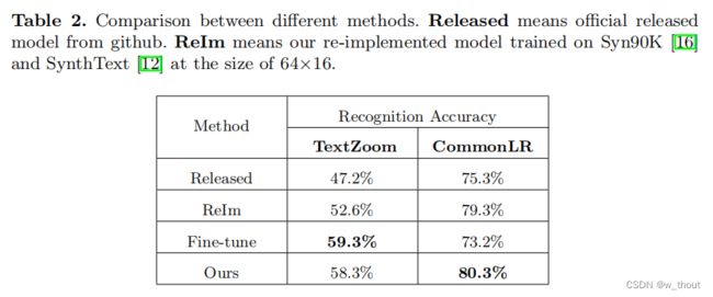
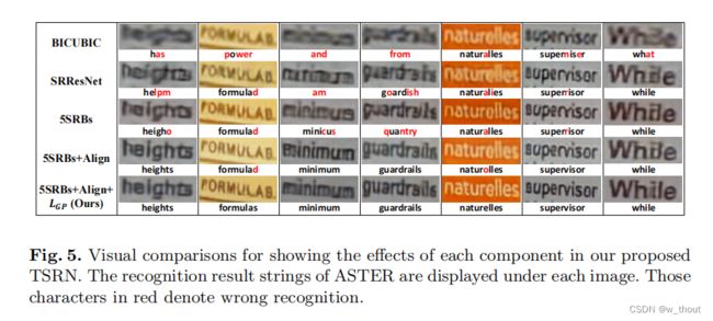
实际上，本文的方法在以下几个方面都优于进行微调和重新调整的方法。 (1)微调后的模型在TextZoom上过度匹配。它在TextZoom上获得了最高的性能，而在CommomomLR上获得了最低的性能，因为TextZoom的数量还远远不足以完成文本识别任务。超分辨率是一项低级别的任务，通常需要更少的数据来收敛。本文的方法可以直接根据尺寸选择SR，并获得更好的整体性能。(2)本文的SR方法也可以产生更好的视觉结果供人们阅读。（图5） (3)re-Im和微调方法需要对大小图像分别建立2个识别模型，而本文的方法只需要一个很小的SR模型，引入了边际计算成本。

因此，SR方法是一种有效、方便的场景文本识别预处理方法。

合成的LR图像 vs TextZoom上的LR图像

在真实LR(TextZoom)数据集上训练的三种方法在精度上明显优于在合成LR上训练的模型。对于本文的TSRN，在真实LR上训练的模型在aster和moran上可以超过合成LR近9.0%，在CRNN上接近14.0%。

TSRN的消融实验

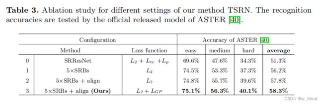
1. SRBs。在SRResNet的基本残差块中添加了BLSTM机制，#0和#1实验。叠加5个SRBs，与SRResNet相比，平均准确率提高4.9%。
2. 中央对齐模块。#1和#2实验。中央对齐模块可将平均精度提高1.5%
3. 梯度剖面损失。#2和#3实验。可以提高0.5%的平均精度。

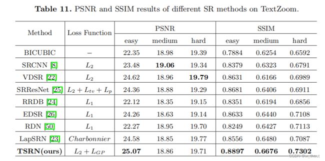
与最先进的SR方法的比较

为了证明TSRN的有效性，本文将其与TextZoom数据集上的7种SISR方法进行了比较，包括SRCNN，VDSR，SRResNet，RRDB，EDSR，RDN和LapSRN。所有的网络都在我们的TextZoom训练集上进行训练，并在我们的三个测试子集上进行评估。

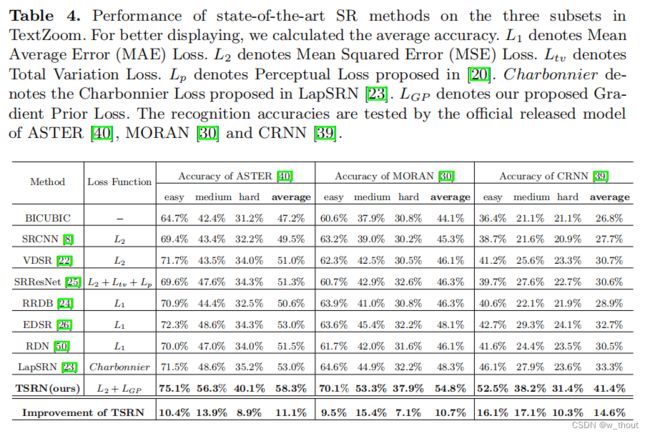
注意SR结果与双三次BICUBIC结果之间的差距。这些方法可以提高平均准确率2.3%∼5.8%，而本文的方法可以提高10.7%∼14.6%。TSRN还可以提高所有三个最先进的识别器的准确性。

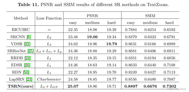
中等子集和难子集的PSNR不是很好，因为PSNR是像素对像素计算的，而SSIM是用11×11滑动核计算的。中央对齐模块会引入轻微的像素位移，因此PSNR比其他SR方法略低。通常，PSNR和SSIM不能代表图像的视觉质量，在这个任务中，它与准确性相比也不那么重要。

结论与讨论

在本工作中验证了场景文本图像超分辨率任务的重要性。本文提出了TextZoom数据集，这是据我们所知的第一个真实配对的场景文本图像超分辨率数据集。TextZoom有很好的注释和分配，并分为三个子集：简单，中等和难。通过大量的实验，本文证明了真实数据比合成数据的优势。为了解决文本图像的超分辨率任务，本文建立了一种新的面向文本的SR方法TSRN。本文的TSRN方法的性能明显优于7种SR方法。这也表明低分辨率文本SR和识别还远未解决，需要更多的研究。
在未来，要捕获更合适的分布式文本图像。非常大的图像和非常小的图像将被避免。图片还应该包含更多的语言，如汉语、法语和德语。还应该重点研究新方法，如将识别注意力引入文本超分辨率任务。

附录

速度与精度

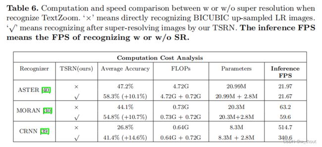
在此任务中，识别精度是最重要的评估度量。为了确定以牺牲TSRN的额外计算消耗为代价来提高精度是否明智，比较了有/无超分辨率的参数、FLOPs和推理FPS的数量。推理FPS是指识别文本图像的FPS。
看到添加TSRN后，基于CTC的识别器CRNN的FPS降低，但精度有很大的提高。因此在识别前加上SR比较好。

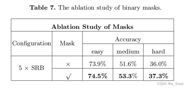
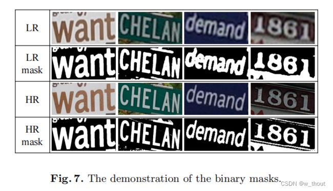
二进制掩码

在文本图像中，字符通常是一个统一的颜色。唯一的纹理信息是字符颜色和背景颜色。将字符区域渲染1，而背景区域渲染0。因为大多数文本图像只包含两种颜色：文本颜色和背景颜色。这些掩模仅仅是通过计算RGB图像的平均灰度来生成的。

关于SRB

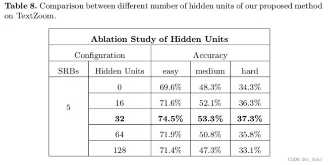
消融实验：1)隐藏的单位。blstm用于在文本行中构建序列依赖性，因此假设更多的隐藏单元可以获得更好的性能。通过实验，比较了0、16、32、64、128个隐藏层。0个隐藏单位表示SRResNet。结果表明，当隐藏单元数量为32时网络可以达到最优性能，过多的隐藏单元性能较低，具有序列依赖性。

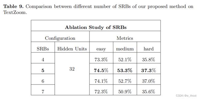
2)块数。为了弄清楚是否可以通过构建更深层次的网络来获得更好的性能，堆叠不同数量的SRB块观察性能。与4、5、6、7个SRB进行了比较。可以发现，更多的SRB可能不会提高性能。7个SRB的精度甚至明显下降。叠加5个SRB，网络饱和，可以获得最好的性能。

SRB块配置：

数据集细节

标注细节

任务分析

一些补充知识

文本识别器ASTER、CRNN、MORAN

OCR文字识别经典论文详解
ASTER文字识别论文详解
文字识别领域经典论文回顾第四期：ASTER
CRNN文字识别

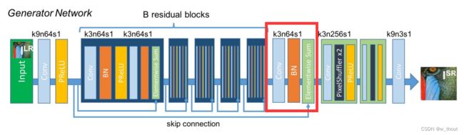
baseline - SRResNet

来源：Photo-Realistic Single Image Super-Resolution Using a Generative Adversarial Network
SRResNet是SRGAN的生成网络部分

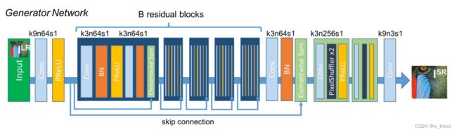
用均方误差优化SRResNet，能够得到具有很高的峰值信噪比的结果。SRResNet部分包含多个残差块，每个残差块中包含两个3×3的卷积层，卷积层后接批规范化层(batch normalization, BN)和PReLU作为激活函数，两个2×亚像素卷积层(sub-pixel convolution layers)被用来增大特征尺寸。

SRB中的双向LSTM（Bi-directional LSTM）

双向 LSTM
双向LSTM和LSTM有什么区别?
LSTM和双向LSTM讲解及实践

中央对齐模块中的

STN（Spatial Transformer Network）

Spatial Transformer Networks
Spatial Transformer Networks
理解Spatial Transformer Networks
论文阅读：Spatial Transformer Networks

Thin-Plate-Spline(TPS)变换

薄板样条插值(Thin Plate Spline)
给定两张图片中一些相互对应的控制点，将其中一个图片进行特定的形变，使得其控制点可以与另一张图片的控制点重合

官方代码阅读

官方代码：JasonBoy1/TextZoom
按readme运行main.py

初始化

main.py中设置了一些参数，命名为args，config中的.yaml文件里也设置了一些参数

if __name__ == '__main__':
    parser = argparse.ArgumentParser(description='')
    parser.add_argument('--arch', default='tsrn', choices=['tsrn', 'bicubic', 'srcnn', 'vdsr', 'srres', 'esrgan', 'rdn',
                                                           'edsr', 'lapsrn'])
    parser.add_argument('--test', action='store_true', default=False)
    parser.add_argument('--test_data_dir', type=str, default='../dataset/lmdb/str/TextZoom/test/medium/', help='')
    parser.add_argument('--batch_size', type=int, default=None, help='')
    parser.add_argument('--resume', type=str, default=None, help='')
    parser.add_argument('--vis_dir', type=str, default=None, help='')
    parser.add_argument('--rec', default='aster', choices=['aster', 'moran', 'crnn'])
    parser.add_argument('--STN', action='store_true', default=False, help='')
    parser.add_argument('--syn', action='store_true', default=False, help='use synthetic LR')
    parser.add_argument('--mixed', action='store_true', default=False, help='mix synthetic with real LR')
    parser.add_argument('--mask', action='store_true', default=False, help='')
    parser.add_argument('--gradient', action='store_true', default=False, help='')
    parser.add_argument('--hd_u', type=int, default=32, help='')
    parser.add_argument('--srb', type=int, default=5, help='')
    parser.add_argument('--demo', action='store_true', default=False)
    parser.add_argument('--demo_dir', type=str, default='./demo')
    args = parser.parse_args()
    config_path = os.path.join('config', 'super_resolution.yaml')
    config = yaml.load(open(config_path, 'r'), Loader=yaml.Loader)
    config = EasyDict(config)
    main(config, args)

在main函数中调用TextSR，该函数在super_resolution.py里，默认执行train，super_resolution.py中定义函数的形参为base.py中的TextBase，TextSR的train里的self来自TextBase函数的定义，从main传给TextSR的实参也在TextBase中赋值。
（device在TextBase中设定）

    def train(self):
        cfg = self.config.TRAIN
        train_dataset, train_loader = self.get_train_data()
        val_dataset_list, val_loader_list = self.get_val_data()
        model_dict = self.generator_init()
        model, image_crit = model_dict['model'], model_dict['crit']

        aster, aster_info = self.Aster_init()
        optimizer_G = self.optimizer_init(model)

train中先是获取了训练集、验证集、初始化SR模型、初始化识别模型、初始化优化器

        if not os.path.exists(cfg.ckpt_dir):
            os.makedirs(cfg.ckpt_dir)
        best_history_acc = dict(
            zip([val_loader_dir.split('/')[-1] for val_loader_dir in self.config.TRAIN.VAL.val_data_dir],
                [0] * len(val_loader_list)))
        best_model_acc = copy.deepcopy(best_history_acc)
        best_model_psnr = copy.deepcopy(best_history_acc)
        best_model_ssim = copy.deepcopy(best_history_acc)
        best_acc = 0
        converge_list = []

然后设置保存中间检查点（历史精度）的文件，做好这些准备工作后开始准备训练。根据epoch按模型训练，并打印epoch信息、精度等。
具体的训练过程在TextBase初始化模型时可以到对应模型的文件中看。

pipeline和SRB

TSRN的forward函数：

  def forward(self, input, source_control_points):
    assert source_control_points.ndimension() == 3
    assert source_control_points.size(1) == self.num_control_points
    assert source_control_points.size(2) == 2
    batch_size = source_control_points.size(0)

    Y = torch.cat([source_control_points, self.padding_matrix.expand(batch_size, 3, 2)], 1)
    mapping_matrix = torch.matmul(self.inverse_kernel, Y)
    source_coordinate = torch.matmul(self.target_coordinate_repr, mapping_matrix)

    grid = source_coordinate.view(-1, self.target_height, self.target_width, 2)
    grid = torch.clamp(grid, 0, 1) # the source_control_points may be out of [0, 1].
    # the input to grid_sample is normalized [-1, 1], but what we get is [0, 1]
    grid = 2.0 * grid - 1.0
    output_maps = grid_sample(input, grid, canvas=None)
    return output_maps, source_coordinate

改进的SRResNet：

in_planes = 3
        if mask:
            in_planes = 4
        assert math.log(scale_factor, 2) % 1 == 0
        upsample_block_num = int(math.log(scale_factor, 2))
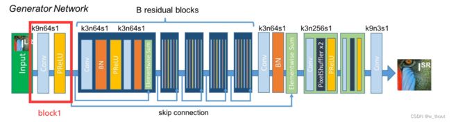
        self.block1 = nn.Sequential(
            nn.Conv2d(in_planes, 2*hidden_units, kernel_size=9, padding=4),
            nn.PReLU()
            # nn.ReLU()
        )

首先设置加上掩码后输入的通道数为4，上采样块的数量取决于缩放因子，设置block1对应SRGAN中生成网络的开头（卷积层+prelu层）

中间有几个基本块，循环设置

self.srb_nums = srb_nums
        for i in range(srb_nums):
            setattr(self, 'block%d' % (i + 2), RecurrentResidualBlock(2*hidden_units))

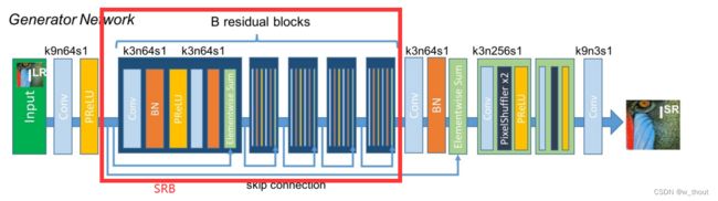
其中的RecurrentResidualBlock是包含两个双向GRU（不知道为什么论文里写的是LSTM但是代码里是GRU）的残差块，看起来好像就是每对卷积和bn层之后直接加了一层双向GRU，具体设置如下

class RecurrentResidualBlock(nn.Module):
    def __init__(self, channels):
        super(RecurrentResidualBlock, self).__init__()
        self.conv1 = nn.Conv2d(channels, channels, kernel_size=3, padding=1)
        self.bn1 = nn.BatchNorm2d(channels)
        self.gru1 = GruBlock(channels, channels)
        # self.prelu = nn.ReLU()
        self.prelu = mish()
        self.conv2 = nn.Conv2d(channels, channels, kernel_size=3, padding=1)
        self.bn2 = nn.BatchNorm2d(channels)
        self.gru2 = GruBlock(channels, channels)

    def forward(self, x):
        residual = self.conv1(x)
        residual = self.bn1(residual)
        residual = self.prelu(residual)
        residual = self.conv2(residual)
        residual = self.bn2(residual)
        residual = self.gru1(residual.transpose(-1, -2)).transpose(-1, -2)
        # residual = self.non_local(residual)

        return self.gru2(x + residual)

双向GRU：

class GruBlock(nn.Module):
    def __init__(self, in_channels, out_channels):
        super(GruBlock, self).__init__()
        assert out_channels % 2 == 0
        self.conv1 = nn.Conv2d(in_channels, out_channels, kernel_size=1, padding=0)
        self.gru = nn.GRU(out_channels, out_channels // 2, bidirectional=True, batch_first=True)

    def forward(self, x):
        x = self.conv1(x)
        x = x.permute(0, 2, 3, 1).contiguous()
        b = x.size()
        x = x.view(b[0] * b[1], b[2], b[3])
        x, _ = self.gru(x)
        # x = self.gru(x)[0]
        x = x.view(b[0], b[1], b[2], b[3])
        x = x.permute(0, 3, 1, 2)
        return x

然后是在SRB之后上采样块之前跟着的一块：

setattr(self, 'block%d' % (srb_nums + 2),
                nn.Sequential(
                    nn.Conv2d(2*hidden_units, 2*hidden_units, kernel_size=3, padding=1),
                    nn.BatchNorm2d(2*hidden_units)
                ))

上采样模块：

class UpsampleBLock(nn.Module):
    def __init__(self, in_channels, up_scale):
        super(UpsampleBLock, self).__init__()
        self.conv = nn.Conv2d(in_channels, in_channels * up_scale ** 2, kernel_size=3, padding=1)

        self.pixel_shuffle = nn.PixelShuffle(up_scale)
        # self.prelu = nn.ReLU()
        self.prelu = mish()

    def forward(self, x):
        x = self.conv(x)
        x = self.pixel_shuffle(x)
        x = self.prelu(x)
        return x

中央对齐模块

STN

原理及代码参考：Spatial Transformer Networks(STN)-代码实现、基于TPS(Thin Plate Spines)的STN网络的PyTorch实现

调用：

		self.tps_inputsize = [32, 64]
        tps_outputsize = [height//scale_factor, width//scale_factor]
        num_control_points = 20   # 在后面的TPS中会用到
        tps_margins = [0.05, 0.05]
        self.stn = STN
        if self.stn:
            self.tps = TPSSpatialTransformer(
                output_image_size=tuple(tps_outputsize),
                num_control_points=num_control_points,
                margins=tuple(tps_margins))

            self.stn_head = STNHead(
                in_planes=in_planes,
                num_ctrlpoints=num_control_points,
                activation='none')
    def forward(self, x):
        # embed()
        if self.stn and self.training:
            x = F.interpolate(x, self.tps_inputsize, mode='bilinear', align_corners=True)
            _, ctrl_points_x = self.stn_head(x)   # 前两个模块
            x, _ = self.tps(x, ctrl_points_x)   # 插值采样
        block = {'1': self.block1(x)}
        for i in range(self.srb_nums + 1):
            block[str(i + 2)] = getattr(self, 'block%d' % (i + 2))(block[str(i + 1)])

        block[str(self.srb_nums + 3)] = getattr(self, 'block%d' % (self.srb_nums + 3)) \
            ((block['1'] + block[str(self.srb_nums + 2)]))
        output = torch.tanh(block[str(self.srb_nums + 3)])
        return output

STN（除TPS）的forward函数：

  def forward(self, x):
    x = self.stn_convnet(x)
    batch_size, _, h, w = x.size()
    x = x.view(batch_size, -1)
    # embed()
    img_feat = self.stn_fc1(x)
    x = self.stn_fc2(0.1 * img_feat)
    if self.activation == 'sigmoid':
      x = F.sigmoid(x)
    x = x.view(-1, self.num_ctrlpoints, 2)
    return img_feat, x

localisation net：从输入图像中提取特征，然后利用全连接层计算基准点参数

  def __init__(self, in_planes, num_ctrlpoints, activation='none'):
    super(STNHead, self).__init__()

    self.in_planes = in_planes
    self.num_ctrlpoints = num_ctrlpoints
    self.activation = activation
     # 提取特征使用的卷积网络
    self.stn_convnet = nn.Sequential(
                          conv3x3_block(in_planes, 32), # 32*64
                          nn.MaxPool2d(kernel_size=2, stride=2),
                          conv3x3_block(32, 64), # 16*32
                          nn.MaxPool2d(kernel_size=2, stride=2),
                          conv3x3_block(64, 128), # 8*16
                          nn.MaxPool2d(kernel_size=2, stride=2),
                          conv3x3_block(128, 256), # 4*8
                          nn.MaxPool2d(kernel_size=2, stride=2),
                          conv3x3_block(256, 256), # 2*4,
                          nn.MaxPool2d(kernel_size=2, stride=2),
                          conv3x3_block(256, 256)) # 1*2
    # 计算基准点使用的两个全连接层
    self.stn_fc1 = nn.Sequential(
                      nn.Linear(2*256, 512),
                      nn.BatchNorm1d(512),
                      nn.ReLU(inplace=True))
    self.stn_fc2 = nn.Linear(512, num_ctrlpoints*2)
    # 初始化卷积层和全连接层 初始化整个网络
    self.init_weights(self.stn_convnet)
    self.init_weights(self.stn_fc1)
    self.init_stn(self.stn_fc2)

  def init_weights(self, module):
    for m in module.modules():
      if isinstance(m, nn.Conv2d):
        n = m.kernel_size[0] * m.kernel_size[1] * m.out_channels
        m.weight.data.normal_(0, math.sqrt(2. / n))
        if m.bias is not None:
          m.bias.data.zero_()
      elif isinstance(m, nn.BatchNorm2d):
        m.weight.data.fill_(1)
        m.bias.data.zero_()
      elif isinstance(m, nn.Linear):
        m.weight.data.normal_(0, 0.001)
        m.bias.data.zero_()

  def init_stn(self, stn_fc2):
    margin = 0.01
    sampling_num_per_side = int(self.num_ctrlpoints / 2)
    ctrl_pts_x = np.linspace(margin, 1.-margin, sampling_num_per_side)
    ctrl_pts_y_top = np.ones(sampling_num_per_side) * margin
    ctrl_pts_y_bottom = np.ones(sampling_num_per_side) * (1-margin)
    ctrl_pts_top = np.stack([ctrl_pts_x, ctrl_pts_y_top], axis=1)
    ctrl_pts_bottom = np.stack([ctrl_pts_x, ctrl_pts_y_bottom], axis=1)
    ctrl_points = np.concatenate([ctrl_pts_top, ctrl_pts_bottom], axis=0).astype(np.float32)
    if self.activation is 'none':
      pass
    elif self.activation == 'sigmoid':
      ctrl_points = -np.log(1. / ctrl_points - 1.)
    stn_fc2.weight.data.zero_()
    stn_fc2.bias.data = torch.Tensor(ctrl_points).view(-1)

TPS

Grid generator、Sampler：写在一个TPS里

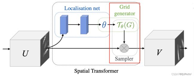
Grid generator是根据上一层的输出变换矩阵进行图片的坐标变换，Sampler是插值采样

class TPSSpatialTransformer(nn.Module):

  def __init__(self, output_image_size=None, num_control_points=None, margins=None):
    super(TPSSpatialTransformer, self).__init__()
    self.output_image_size = output_image_size
    self.num_control_points = num_control_points
    self.margins = margins

    self.target_height, self.target_width = output_image_size
    target_control_points = build_output_control_points(num_control_points, margins)
    N = num_control_points
    # N = N - 4

    # create padded kernel matrix
    forward_kernel = torch.zeros(N + 3, N + 3)
    target_control_partial_repr = compute_partial_repr(target_control_points, target_control_points)
    forward_kernel[:N, :N].copy_(target_control_partial_repr)
    forward_kernel[:N, -3].fill_(1)
    forward_kernel[-3, :N].fill_(1)
    forward_kernel[:N, -2:].copy_(target_control_points)
    forward_kernel[-2:, :N].copy_(target_control_points.transpose(0, 1))
    # compute inverse matrix
    inverse_kernel = torch.inverse(forward_kernel)

    # create target cordinate matrix
    HW = self.target_height * self.target_width
    target_coordinate = list(itertools.product(range(self.target_height), range(self.target_width)))
    target_coordinate = torch.Tensor(target_coordinate) # HW x 2
    Y, X = target_coordinate.split(1, dim = 1)
    Y = Y / (self.target_height - 1)
    X = X / (self.target_width - 1)
    target_coordinate = torch.cat([X, Y], dim = 1) # convert from (y, x) to (x, y)
    target_coordinate_partial_repr = compute_partial_repr(target_coordinate, target_control_points)
    target_coordinate_repr = torch.cat([
      target_coordinate_partial_repr, torch.ones(HW, 1), target_coordinate
    ], dim = 1)

    # register precomputed matrices
    self.register_buffer('inverse_kernel', inverse_kernel)
    self.register_buffer('padding_matrix', torch.zeros(3, 2))
    self.register_buffer('target_coordinate_repr', target_coordinate_repr)
    self.register_buffer('target_control_points', target_control_points)
  def forward(self, input, source_control_points):
    assert source_control_points.ndimension() == 3
    assert source_control_points.size(1) == self.num_control_points
    assert source_control_points.size(2) == 2
    batch_size = source_control_points.size(0)

    Y = torch.cat([source_control_points, self.padding_matrix.expand(batch_size, 3, 2)], 1)
    mapping_matrix = torch.matmul(self.inverse_kernel, Y)
    source_coordinate = torch.matmul(self.target_coordinate_repr, mapping_matrix)

    grid = source_coordinate.view(-1, self.target_height, self.target_width, 2)
    grid = torch.clamp(grid, 0, 1) # the source_control_points may be out of [0, 1].
    # the input to grid_sample is normalized [-1, 1], but what we get is [0, 1]
    grid = 2.0 * grid - 1.0
    # 采样
    output_maps = grid_sample(input, grid, canvas=None)
    return output_maps, source_coordinate

采样的函数定义：

def grid_sample(input, grid, canvas = None):
  output = F.grid_sample(input, grid)
  if canvas is None:
    return output
  else:
    input_mask = input.data.new(input.size()).fill_(1)
    output_mask = F.grid_sample(input_mask, grid)
    padded_output = output * output_mask + canvas * (1 - output_mask)
    return padded_output

网格变换函数定义：

# phi(x1, x2) = r^2 * log(r), where r = ||x1 - x2||_2
def compute_partial_repr(input_points, control_points):
  N = input_points.size(0)
  M = control_points.size(0)
  pairwise_diff = input_points.view(N, 1, 2) - control_points.view(1, M, 2)
  # original implementation, very slow
  # pairwise_dist = torch.sum(pairwise_diff ** 2, dim = 2) # square of distance
  pairwise_diff_square = pairwise_diff * pairwise_diff
  pairwise_dist = pairwise_diff_square[:, :, 0] + pairwise_diff_square[:, :, 1]
  repr_matrix = 0.5 * pairwise_dist * torch.log(pairwise_dist)
  # fix numerical error for 0 * log(0), substitute all nan with 0
  mask = repr_matrix != repr_matrix
  repr_matrix.masked_fill_(mask, 0)
  return repr_matrix


# output_ctrl_pts are specified, according to our task.
def build_output_control_points(num_control_points, margins):
  margin_x, margin_y = margins
  num_ctrl_pts_per_side = num_control_points // 2
  ctrl_pts_x = np.linspace(margin_x, 1.0 - margin_x, num_ctrl_pts_per_side)
  ctrl_pts_y_top = np.ones(num_ctrl_pts_per_side) * margin_y
  ctrl_pts_y_bottom = np.ones(num_ctrl_pts_per_side) * (1.0 - margin_y)
  ctrl_pts_top = np.stack([ctrl_pts_x, ctrl_pts_y_top], axis=1)
  ctrl_pts_bottom = np.stack([ctrl_pts_x, ctrl_pts_y_bottom], axis=1)
  # ctrl_pts_top = ctrl_pts_top[1:-1,:]
  # ctrl_pts_bottom = ctrl_pts_bottom[1:-1,:]
  output_ctrl_pts_arr = np.concatenate([ctrl_pts_top, ctrl_pts_bottom], axis=0)
  output_ctrl_pts = torch.Tensor(output_ctrl_pts_arr)
  return output_ctrl_pts

损失计算

如果不加梯度损失就只用mse（L2）损失，如果要加就加上梯度先验损失

class ImageLoss(nn.Module):
    def __init__(self, gradient=True, loss_weight=[20, 1e-4]):
        super(ImageLoss, self).__init__()
        self.mse = nn.MSELoss()
        if gradient:
            self.GPLoss = GradientPriorLoss()
        self.gradient = gradient
        self.loss_weight = loss_weight

    def forward(self, out_images, target_images):
        if self.gradient:
            loss = self.loss_weight[0] * self.mse(out_images, target_images) + \
                   self.loss_weight[1] * self.GPLoss(out_images[:, :3, :, :], target_images[:, :3, :, :])
        else:
            loss = self.loss_weight[0] * self.mse(out_images, target_images)
        return loss


class GradientPriorLoss(nn.Module):
    def __init__(self, ):
        super(GradientPriorLoss, self).__init__()
        self.func = nn.L1Loss()

    def forward(self, out_images, target_images):
        map_out = self.gradient_map(out_images)
        map_target = self.gradient_map(target_images)
        return self.func(map_out, map_target)

    @staticmethod
    def gradient_map(x):
        batch_size, channel, h_x, w_x = x.size()
        r = F.pad(x, (0, 1, 0, 0))[:, :, :, 1:]
        l = F.pad(x, (1, 0, 0, 0))[:, :, :, :w_x]
        t = F.pad(x, (0, 0, 1, 0))[:, :, :h_x, :]
        b = F.pad(x, (0, 0, 0, 1))[:, :, 1:, :]
        xgrad = torch.pow(torch.pow((r - l) * 0.5, 2) + torch.pow((t - b) * 0.5, 2)+1e-6, 0.5)
        return xgrad

GP损失定义如下：

总结——文本超分及识别流程图（以官方代码为基础）

PSNR

PSNR计算：【python】psnr原理简介及代码实现
流程图：

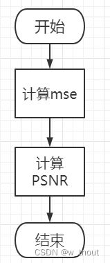
mse：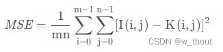
psnr：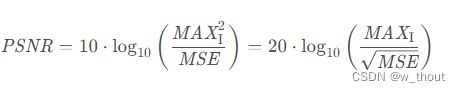

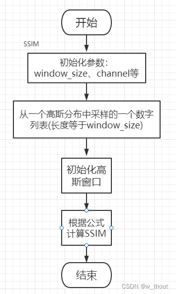
SSIM

SSIM原理及代码：结构相似度索引（SSIM）全攻略：理论+代码（PyTorch）、SSIM (Structure Similarity Index Measure) 结构衡量指标+代码、深入理解SSIM(两图像结构相似度指标)(附matlab代码)

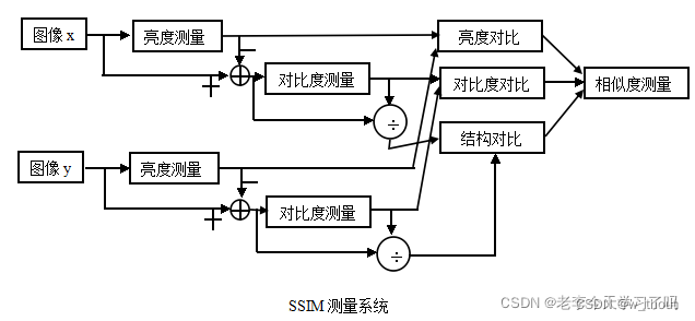
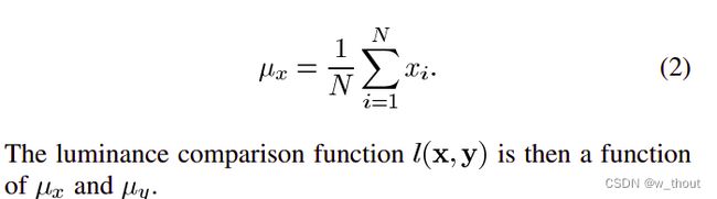
亮度：亮度通过对所有像素值进行平均测量。用μ表示，公式如下：

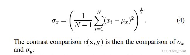
对比度：取所有像素值的标准差(方差的平方根)来测量。用σ表示，表示为：

结构：结构比较是通过使用一个合并公式来完成的(后面会详细介绍)，但在本质上，我们用输入信号的标准差来除以它，因此结果有单位标准差，这可以得到一个更稳健的比较。

亮度比较函数：由函数定义，l(x, y)，如下图所示。μ表示给定图像的平均值。x和y是被比较的两个图像。

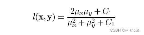
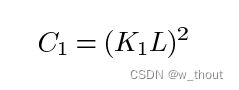
其中C1为常数，保证分母为0时的稳定性。C1这样给出：

对比度比较函数：由函数c(x, y)定义，如下图所示。σ表示给定图像的标准差。x和y是被比较的两个图像。

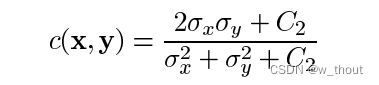
其中C2这样给出：

结构比较函数：由函数s(x, y)定义，如下图所示。σ表示给定图像的标准差。x和y是被比较的两个图像。

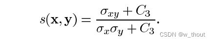
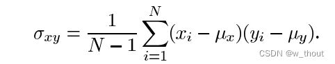
其中σ(xy)定义为：

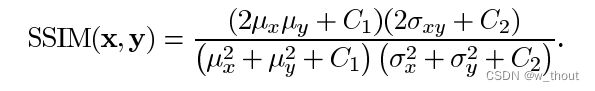
最后，SSIM定义为：

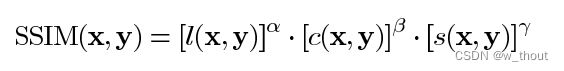
其中 α > 0, β > 0, γ > 0 表示每个度量标准的相对重要性。为了简化表达式，我们设：

实际上，当需要衡量一整张图片的质量，经常使用的是以一个一个窗口计算SSIM然后求平均。
当我们用一个一个block去计算平均值，标准差，协方差时，这种方法容易造成 blocking artifacts, 所以在计算MSSIM时，会使用到 circular-symmetric Gaussian weighting function圆对称的高斯加权公式 ​​, 标准差为1.5，和为1，来估计局部平均值，标准差，协方差。由于我们现在在局部计算，我们的公式被修改为：

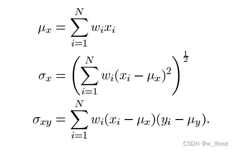
其中wi是高斯加权函数。
流程图：

数据初始化

从文件夹中获取对应训练集和测试集后需要进行数据初始化，在初始化时会对图像进行一次对齐操作，通过标准化resize图像完成，其流程如下：
流程：

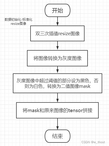
hr和lr都要进行该操作，lr时需要将原图像除以下采样因子