图像分类经典卷积神经网络—ZFNet论文翻译（中英文对照版）—Visualizing and Understanding Convolutional Networks(可视化和理解卷积网络)

图像分类经典论文翻译汇总：[翻译汇总]

翻译pdf文件下载：[下载地址]

此版为中英文对照版，纯中文版请稳步：[ZFNet纯中文版]

Visualizing and Understanding Convolutional Networks 可视化和理解卷积网络
Matthew D. Zeiler		Rob Fergus
Dept. of Computer Science, New York University, USA（美国纽约大学计算机科学系） {zeiler,fergus}@cs.nyu.edu

Abstract

Large Convolutional Network models have recently demonstrated impressive classification performance on the ImageNet benchmark Krizhevsky et al. [18]. However there is no clear understanding of why they perform so well, or how they might be improved. In this paper we explore both issues. We introduce a novel visualization technique that gives insight into the function of intermediate feature layers and the operation of the classifier. Used in a diagnostic role, these visualizations allow us to find model architectures that outperform Krizhevsky et al. on the ImageNet classification benchmark. We also perform an ablation study to discover the performance contribution from different model layers. We show our ImageNet model generalizes well to other datasets: when the softmax classifier is retrained, it convincingly beats the current state-of-the-art results on Caltech-101 and Caltech-256 datasets.

摘要

大型卷积网络模型最近在ImageNet基准测试上表现出了令人印象深刻的分类性能Krizhevsky等[18]。然而，人们还没有明确的理解他们为什么表现如此之好，或者如何改进它们。在本文中，我们将探讨这两个问题。我们介绍了一种新的可视化技术，可以深入了解中间特征层的功能和分类器的操作。作为诊断的手段，这些可视化技术使我们能够找到优于Krizhevsky等人在ImageNet分类基准的模型架构。我们还进行了消融研究，以发现不同模型层的在模型性能上的贡献。我们的研究表明我们的ImageNet模型能很好地泛化到其他数据集：当softmax分类器被重新训练时，它令人信服地击败了Caltech-101和Caltech-256数据集上当前最先进的结果。

1 Introduction

Since their introduction by LeCun et al. [20] in the early 1990’s, Convolutional Networks (convnets) have demonstrated excellent performance at tasks such as hand-written digit classification and face detection. In the last 18 months, several papers have shown that they can also deliver outstanding performance on more challenging visual classification tasks. Ciresan et al. [4] demonstrate state-of-the-art performance on NORB and CIFAR-10 datasets. Most notably, Krizhevsky et al. [18] show record beating performance on the ImageNet 2012 classification benchmark, with their convnet model achieving an error rate of 16.4%, compared to the 2nd place result of 26.1%. Following on from this work, Girshick et al. [10] have shown leading detection performance on the PASCAL VOC dataset. Several factors are responsible for this dramatic improvement in performance: (i) the availability of much larger training sets, with millions of labeled examples; (ii) powerful GPU implementations, making the training of very large models practical and (iii) better model regularization strategies, such as Dropout [14].

1 引言

自20世纪90年代早期LeCun等[20]提出卷积网络以来，卷积网络（convnets）在手写数字分类和人脸检测等任务中表现出色。在过去的18个月中，有几篇论文表明，他们还可以在更具挑战性的视觉分类任务中具有更出色的表现。Ciresan等[4]表明其在NORB和CIFAR-10数据集上最好的性能。最值得注意的是，Krizhevsky等[18]在ImageNet 2012分类基准测试中获得了创纪录的表现，他们的卷积模型实现了16.4％的错误率，而第二名的结果是26.1％。基于这项研究工作，Girshick等[10]研究报道了PASCAL VOC数据集上最佳的检测性能。有几个因素导致这种性能的显着提高：（i）具有数百万个标记样本的更大规模的训练集的可用性;（ii）强大的GPU实现，使非常大的模型的训练成为现实;（iii）更好的模型正则化策略，例如Dropout [14]。

Despite this encouraging progress, there is still little insight into the internal operation and behavior of these complex models, or how they achieve such good performance. From a scientific standpoint, this is deeply unsatisfactory. Without clear understanding of how and why they work, the development of better models is reduced to trial-and-error. In this paper we introduce a visualization technique that reveals the input stimuli that excite individual feature maps at any layer in the model. It also allows us to observe the evolution of features during training and to diagnose potential problems with the model. The visualization technique we propose uses a multi-layered Deconvolutional Network (deconvnet), as proposed by Zeiler et al. [29], to project the feature activations back to the input pixel space. We also perform a sensitivity analysis of the classifier output by occluding portions of the input image, revealing which parts of the scene are important for classification.

尽管取得了令人鼓舞的进展，但对这些复杂模型的内部操作和行为，或者它们如何实现如此良好的性能，仍然了解甚少。从科学的角度来看，这是非常令人不满意的。如果没有清楚地了解它们如何以及为何起作用，那么更好的模型的开发过程将被简化为试错。在本文中，我们介绍了一种可视化技术，该技术揭示了激发模型中任何层的单个特征映射的输入激励。它还允许我们在训练期间观察特征的演变并诊断模型的潜在问题。我们提出的可视化技术使用Zeiler等[29]提出的多层反卷积网络（deconvnet），即将特征激活投影回输入像素空间。我们还通过遮挡输入图像的部分来进行分类器输出的灵敏度分析，从而揭示图像的哪些部分对于分类是重要的。

Using these tools, we start with the architecture of Krizhevsky et al. [18] and explore different architectures, discovering ones that outperform their results on ImageNet. We then explore the generalization ability of the model to other datasets, just retraining the softmax classifier on top. As such, this is a form of supervised pre-training, which contrasts with the unsupervised pre-training methods popularized by Hinton et al. [13] and others [1,26].

使用这些工具，我们从Krizhevsky等[18]的架构开始，探索不同的架构，发现在ImageNet上超越其结果的架构。然后，我们探索模型对其他数据集的泛化能力，只需重新训练softmax分类器。因此，这是一种受监督的预训练形式，这不同于Hinton等[13]和其他人[1,26]推广的无监督预训练方法。

1.1 Related Work

Visualization: Visualizing features to gain intuition about the network is common practice, but mostly limited to the 1st layer where projections to pixel space are possible. In higher layers alternate methods must be used. [8] find the optimal stimulus for each unit by performing gradient descent in image space to maximize the unit’s activation. This requires a careful initialization and does not give any information about the unit’s invariances. Motivated by the latter’s short-coming, [19] (extending an idea by [2]) show how the Hessian of a given unit may be computed numerically around the optimal response, giving some insight into invariances. The problem is that for higher layers, the invariances are extremely complex so are poorly captured by a simple quadratic approximation. Our approach, by contrast, provides a non-parametric view of invariance, showing which patterns from the training set activate the feature map. Our approach is similar to contemporary work by Simonyan et al. [23] who demonstrate how saliency maps can be obtained from a convnet by projecting back from the fully connected layers of the network, instead of the convolutional features that we use. Girshick et al. [10] show visualizations that identify patches within a dataset that are responsible for strong activations at higher layers in the model. Our visualizations differ in that they are not just crops of input images, but rather top-down projections that reveal structures within each patch that stimulate a particular feature map.

1.1 相关工作

可视化：可视化特征以获得关于网络的直觉是常见的做法，但主要局限于可以投影到像素空间第一层。在较高层中，必须使用其它方法。[8]通过在图像空间中执行梯度下降来找到每个单元的最佳刺激，以最大化单元的激活。这需要谨慎的初始化，并且不提供有关单元不变量的任何信息。由后者的缺点所激发，[19]（通过[2]扩展一个想法）揭示如何围绕最优响应以数字方式计算给定单元的Hessian矩阵，从而对不变量有所了解。问题是对于更高层，不变量非常复杂，因此通过简单的二次近似很难捕获。相反，我们的方法提供了不变量的非参数视图，显示了训练集中的哪些模式激活了特征映射。我们的方法类似于Simonyan等[23]同期工作，他们揭示了如何通过从网络的全连接层投影回来而获得显着性图，而不是我们使用的卷积特征。Girshick等[10]表明识别数据集中的补丁的可视化，这些补丁与模型中较高层的强激活相关。我们的可视化不同之处在于它们不仅仅是输入图像的裁剪，而是自上而下的投影，揭示每个图像块中刺激特定特征图的结构。

Feature Generalization: Our demonstration of the generalization ability of convnet features is also explored in concurrent work by Donahue et al. [7] and Girshick et al. [10]. They use the convnet features to obtain state-of-the-art performance on Caltech-101 and the Sun scenes dataset in the former case, and for object detection on the PASCAL VOC dataset, in the latter.

特征泛化：在Donahue等[7]和Girshick等[10]的同期工作中也探讨了我们研究的卷积特征的泛化能力。他们使用卷积特征在前一个研究中获得Caltech-101和Sun场景数据集的最佳性能，后者研究是在PASCAL VOC数据集上进行对象检测。

2 Approach

We use standard fully supervised convnet models throughout the paper, as defined by LeCun et al. [20] and Krizhevsky et al. [18]. These models map a color 2D input image xi, via a series of layers, to a probability vector yi over the C different classes. Each layer consists of (i) convolution of the previous layer output (or, in the case of the 1st layer, the input image) with a set of learned filters; (ii) passing the responses through a rectified linear function (relu(x) = max(x, 0)); (iii) [optionally] max pooling over local neighborhoods and (iv) [optionally] a local contrast operation that normalizes the responses across feature maps. For more details of these operations, see [18] and [16]. The top few layers of the network are conventional fully-connected networks and the final layer is a softmax classifier. Fig. 3 shows the model used in many of our experiments.

2 方法

根据LeCun及Krizhevsky等的定义，我们在整篇论文中使用标准的完全监督的卷积模型。这些模型通过一系列层将彩色2D输入图像xi映射到C个不同类别上的概率向量yi。每层包括：（i）前一层输出（或在第一层的情况下，输入图像）与一组学习过滤器的卷积; （ii）通过整流线性函数（relu(x) = max(x，0)）传递响应；（iii）[可选地]在局部邻域上的最大池化和（iv）[可选地]局部对比操作，其对特征映射之间的响应进行归一化。有关这些操作的更多详细信息，请参见[18]和[16]。网络的前几层是传统的全连接网络，最后一层是softmax分类器。图3显示了我们许多实验中使用的模型。

We train these models using a large set of N labeled images {x, y}, where label yi is a discrete variable indicating the true class. A cross-entropy loss function, suitable for image classification, is used to compare yi and yi. The parameters of the network (filters in the convolutional layers, weight matrices in the fully-connected layers and biases) are trained by back-propagating the derivative of the loss with respect to the parameters throughout the network, and updating the parameters via stochastic gradient descent. Details of training are given in Section 3.

我们使用大量N个标记图像{x，y}训练这些模型，其中标签yi是指示真实类的离散变量。适用于图像分类的交叉熵损失函数用于比较yi和yi。网络的参数（卷积层中的滤波器，全连接层中的权重矩阵和偏差）通过相对于整个网络中的参数反向传播损耗的导数来训练，并通过随机梯度下降来更新参数。训练的详细情节见第3部分。

2.1 Visualization with a Deconvnet

Understanding the operation of a convnet requires interpreting the feature activity in intermediate layers. We present a novel way to map these activities back to the input pixel space, showing what input pattern originally caused a given activation in the feature maps. We perform this mapping with a Deconvolutional Network (deconvnet) Zeiler et al. [29]. A deconvnet can be thought of as a convnet model that uses the same components (filtering, pooling) but in reverse, so instead of mapping pixels to features does the opposite. In Zeiler et al. [29], deconvnets were proposed as a way of performing unsupervised learning. Here, they are not used in any learning capacity, just as a probe of an already trained convnet.

2.1 通过反卷积可视化

理解卷积网络的操作需要解释中间层的特征活动。我们提出了一种新颖的方法来将这些活动映射回输入像素空间，显示最初在特征映射中引起给定激活的输入模式。我们使用反卷积网络（deconvnet）Zeiler等[29]实现此映射。反卷积网络可以被认为是一个使用相同组件（过滤，池化）的逆向的卷积模型，即不是将像素映射到特征，而是将特征映射到像素。在Zeiler等[29]中，反卷积网络作为进行无监督学习的一种方式而被提出。在这里，它们不会用于任何学习能力，仅作为对已经训练好的卷积网络的探索。

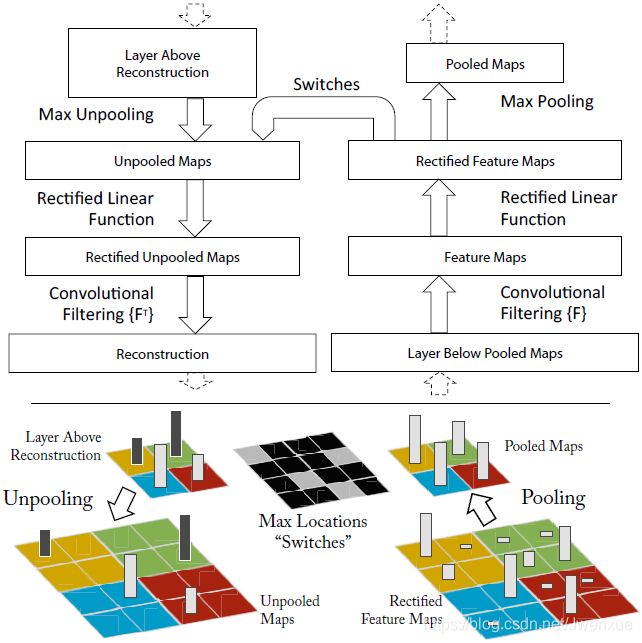
To examine a convnet, a deconvnet is attached to each of its layers, as illustrated in Fig. 1(top), providing a continuous path back to image pixels. To start, an input image is presented to the convnet and features computed throughout the layers. To examine a given convnet activation, we set all other activations in the layer to zero and pass the feature maps as input to the attached deconvnet layer. Then we successively (i) unpool, (ii) rectify and (iii) filter to reconstruct the activity in the layer beneath that gave rise to the chosen activation. This is then repeated until input pixel space is reached.

Fig. 1. Top: A deconvnet layer (left) attached to a convnet layer (right). The deconvnet will reconstruct an approximate version of the convnet features from the layer beneath. Bottom: An illustration of the unpooling operation in the deconvnet, using switches which record the location of the local max in each pooling region (colored zones) during pooling in the convnet. The black/white bars are negative/positive activations within the feature map.

如图1（上图）所示，为了检查一个卷积网络，网络的每个层都附有一个反卷积网络，提供了一条返回图像像素的连续路径。首先，将输入图像呈现给卷积网络并通过所有层计算特征。为了检查给定卷积网络的激活，我们将图层中的所有其他激活设置为零，并将特征图作为输入传递给附加的反卷积网络层。然后我们依次（i）反池化，（ii）纠正和（iii）过滤以重建下面的层中的活动，从而产生所选择的激活。 然后重复这一过程，直到达到输入像素空间。

图1.上图：反卷积层（左）与卷积层（右）相连。反卷积网络将从下面的层重建一个近似版本的卷积网络特征。下图：反卷积网络中使用switch反池化操作的示意图，switch记录卷积网络池化时每个池化区域（彩色区域）中局部最大值的位置。黑/白条在特征图中表示负/正激活。

Unpooling: In the convnet, the max pooling operation is non-invertible, however we can obtain an approximate inverse by recording the locations of the maxima within each pooling region in a set of switch variables. In the deconvnet, the unpooling operation uses these switches to place the reconstructions from the layer above into appropriate locations, preserving the structure of the stimulus. See Fig. 1(bottom) for an illustration of the procedure.

反池化：在卷积网络中，最大池化操作是不可逆的，但是我们可以通过在一组切换变量中记录每个池化区域内的最大值的位置来获得近似逆。在反卷积网络中，反池化操作使用这些切换将来自上层的重建放置到适当的位置，从而保留激活的结构。有关步骤的插图，请参见图1（底部）。

Rectification: The convnet uses relu non-linearities, which rectify the feature maps thus ensuring the feature maps are always positive. To obtain valid feature reconstructions at each layer (which also should be positive), we pass the reconstructed signal through a relu non-linearity1.

纠正：卷积网络使用relu的非线性，即纠正特征图，从而确保特征图始终为正。为了在每一层获得有效的特征重建（也应该是正的），我们通过relu非线性传递重建的信号。

Filtering: The convnet uses learned filters to convolve the feature maps from the previous layer. To approximately invert this, the deconvnet uses transposed versions of the same filters (as other autoencoder models, such as RBMs), but applied to the rectified maps, not the output of the layer beneath. In practice this means flipping each filter vertically and horizontally.

滤波：卷积网络使用学习到的过滤器来卷积前一层的特征图。为了近似反转这一点，反卷积网络使用相同滤波器的转置版本（如其他自动编码器模型，例如RBM），但应用于纠正的映射图，而不是层下面的输出。实际上，这意味着垂直和水平翻转每个过滤器。

Note that we do not use any contrast normalization operations when in this reconstruction path. Projecting down from higher layers uses the switch settings generated by the max pooling in the convnet on the way up. As these switch settings are peculiar to a given input image, the reconstruction obtained from a single activation thus resembles a small piece of the original input image, with structures weighted according to their contribution toward to the feature activation. Since the model is trained discriminatively, they implicitly show which parts of the input image are discriminative. Note that these projections are not samples from the model, since there is no generative process involved. The whole procedure is similar to backpropping a single strong activation (rather than the usual gradients), i.e. computing ∂h∂Xn, where h is the element of the feature map with the strong activation and Xn is the input image. However, it differs in that (i) the relu is imposed independently and (ii) contrast normalization operations are not used. A general shortcoming of our approach is that it only visualizes a single activation, not the joint activity present in a layer. Nevertheless, as we show in Fig. 6, these visualizations are accurate representations of the input pattern that stimulates the given feature map in the model: when the parts of the original input image corresponding to the pattern are occluded, we see a distinct drop in activity within the feature map.

请注意，在此重建路径中，我们没有使用任何对比度归一化操作。从较高层向下投影使用在前进途中由卷积网络中的最大池化生成的切换设置。由于这些开关设置是给定输入图像所特有的，因此从单次激活获得的重建类似于原始输入图像的一小块，其结构根据它们对特征激活的贡献而加权。由于模型是有区别地训练的，因此它们隐含地表明输入图像的哪些部分是有区别的。请注意，这些预测不是来自模型的样本，因为不涉及生成过程。整个过程类似于反向支持单个强激活（而不是通常的梯度），即计算∂h∂Xn，其中h是具有强激活的特征映射的元素，而Xn是输入图像。然而，它的不同之处在于（i）独立地施加relu，（ii）不使用对比度归一化操作。我们的方法的一个总体缺点是它只能显示单个激活，而不是图层中存在的整体的激活。然而，正如我们在图6中所示，这些可视化是输入模式的精确表示，其刺激模型中的给定特征图：当对应于模式的原始输入图像的部分被遮挡时，我们看到特征图中激活的明显下降。

3 Training Details

We now describe the large convnet model that will be visualized in Section 4. The architecture, shown in Fig. 3, is similar to that used by Krizhevsky et al. [18] for ImageNet classification. One difference is that the sparse connections used in Krizhevsky’s layers 3,4,5 (due to the model being split across 2 GPUs) are replaced with dense connections in our model. Other important differences relating to layers 1 and 2 were made following inspection of the visualizations in Fig. 5, as described in Section 4.1.

3 训练细节

我们现在描述将在第4节中被可视化的大型卷积网络模型。图3中所示的架构类似于Krizhevsky等[18]用于ImageNet分类的架构。一个区别是Krizhevsky的3,4,5层使用的稀疏连接（由于模型分为2个GPU）在我们的模型中被密集连接替换。另一个重要的不同是关于1，2层，其被用于图5中后面可视化的检查，如4.1部分所述。

The model was trained on the ImageNet 2012 training set (1.3 million images, spread over 1000 different classes) [6]. Each RGB image was preprocessed by resizing the smallest dimension to 256, cropping the center 256×256 region, subtracting the per-pixel mean (across all images) and then using 10 different sub-crops of size 224×224 (corners + center with(out) horizontal flips). Stochastic gradient descent with a mini-batch size of 128 was used to update the parameters, starting with a learning rate of 10−2, in conjunction with a momentum term of 0.9. We anneal the learning rate throughout training manually when the validation error plateaus. Dropout [14] is used in the fully connected layers (6 and 7) with a rate of 0.5. All weights are initialized to 10−2 and biases are set to 0.

该模型在ImageNet 2012训练集上进行了训练（130万张图像，分布在1000多个不同的类别中）[6]。每个RGB图像都经过预处理，方法是将最小尺寸调整为256，裁剪中心256×256区域，减去像素平均值（在所有图像上），然后得到10个不同的裁剪块，尺寸为224×224（原图像及水平翻转的四个角+中心）。使用具有128的小批量大小的随机梯度下降来更新参数，学习率10-2开始，结合动量项0.9。当验证错误达到平稳时，我们在整个训练过程中手动降低学习率。Dropout [14]用于全连接的层（6，7层），dropout比率为0.5。所有权重都初始化为10-2，偏差设置为0。

Visualization of the first layer filters during training reveals that a few of them dominate. To combat this, we renormalize each filter in the convolutional layers whose RMS value exceeds a fixed radius of 10−1 to this fixed radius. This is crucial, especially in the first layer of the model, where the input images are roughly in the [-128, 128] range. As in Krizhevsky et al. [18], we produce multiple different crops and flips of each training example to boost training set size. We stopped training after 70 epochs, which took around 12 days on a single GTX580 GPU, using an implementation based on [18].

在训练期间可视化第一层过滤器显示其中一些过滤器占主导地位。为了解决这个问题，我们将其RMS值超过固定半径10-1的卷积层中的每个滤波器重新归一化到该固定半径。这一点至关重要，特别是在模型的第一层，输入图像大致在[-128, 128]范围内。如在Krizhevsky等[18]，我们生成了多种不同的裁剪块和每个训练样例的翻转，以提高训练集的大小。我们在70个epochs之后停止了训练，基于[18]的实现在一个GTX580 GPU上花了大约12天。

4 Convnet Visualization

Using the model described in Section 3, we now use the deconvnet to visualize the feature activations on the ImageNet validation set.

4 卷积网络可视化

使用第3节中描述的模型，我们现在使用反卷积网络可视化ImageNet验证集上的特征激活。

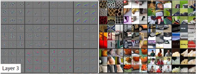
Feature Visualization: Fig. 2 shows feature visualizations from our model once training is complete. For a given feature map, we show the top 9 activations, each projected separately down to pixel space, revealing the different structures that excite that map and showing its invariance to input deformations. Alongside these visualizations we show the corresponding image patches. These have greater variation than visualizations which solely focus on the discriminant structure within each patch. For example, in layer 5, row 1, col 2, the patches appear to have little in common, but the visualizations reveal that this particular feature map focuses on the grass in the background, not the foreground objects.

Fig. 2. Visualization of features in a fully trained model. For layers 2-5 we show the top 9 activations in a random subset of feature maps across the validation data, projected down to pixel space using our deconvolutional network approach. Our reconstructions are not samples from the model: they are reconstructed patterns from the validation set that cause high activations in a given feature map. For each feature map we also show the corresponding image patches. Note: (i) the strong grouping within each feature map, (ii) greater invariance at higher layers and (iii) exaggeration of discriminative parts of the image, e.g. eyes and noses of dogs (layer 4, row 1, cols 1). Best viewed in electronic form. The compression artifacts are a consequence of the 30Mb submission limit, not the reconstruction algorithm itself.

特征可视化：图2所示为训练完成后我们模型的特征可视化。对于给定的特征映射，我们显示前9个激活，每个激活分别投影到像素空间，揭示激发该映射并显示其对输入变形的不变性的不同结构。 除了这些可视化外，我们还会显示相应的图像补丁。 它们比可视化具有更大的变化，可视化仅关注每个补丁内的判别结构。 例如，在第5层，第1行，第2列中，补丁似乎没有什么共同之处，但可视化显示此特定要素图聚焦于背景中的草，而不是前景对象。

图2.完全训练模型中的特征可视化。对于2-5层，我们在验证数据的特征映射的随机子集中显示前9个激活，使用我们的反卷积网络方法投影到像素空间。我们的重建不是来自模型的样本：它们是来自验证集的重建模式，其导致给定特征图中的高激活。对于每个特征图，我们还会显示相应的图像块。注意：（i）每个特征图内的强分组，（ii）较高层的较大不变性和（iii）图像的辨别部分的放大，例如，狗的眼睛和鼻子（第4层第1行第1列）。电子版观看效果最佳。由于30Mb的提交限制而使用了压缩算法，而不是重建算法本身。

The projections from each layer show the hierarchical nature of the features in the network. Layer 2 responds to corners and other edge/color conjunctions. Layer 3 has more complex invariances, capturing similar textures (e.g. mesh patterns (Row 1, Col 1); text (R2,C4)). Layer 4 shows significant variation, and is more class-specific: dog faces (R1,C1); bird’s legs (R4,C2). Layer 5 shows entire objects with significant pose variation, e.g. keyboards (R1,C11) and dogs (R4).

每层的投影显示了网络中特征的分层特性。 第2层响应角落和其他边缘/颜色连接。 第3层具有更复杂的不变性，捕获相似的纹理（例如网格图案（第1行，第1列）;文本（R2，C4））。 第4层显示出显着的变化，并且更具有特定类别：狗脸（R1，C1）; 鸟的腿（R4，C2）。 第5层显示具有显着姿势变化的整个对象，例如， 键盘（R1，C11）和狗（R4）。

Feature Evolution during Training: Fig. 4 visualizes the progression during training of the strongest activation (across all training examples) within a given feature map projected back to pixel space. Sudden jumps in appearance result from a change in the image from which the strongest activation originates. The lower layers of the model can be seen to converge within a few epochs. However, the upper layers only develop develop after a considerable number of epochs (40-50), demonstrating the need to let the models train until fully converged.

训练期间的特征演变：图4显示了在投射回像素空间的给定特征图内的最强激活（跨越所有训练示例）的训练期间的进展。 外观突然跳跃是由最强激活源自的图像变化引起的。 可以看到模型的较低层在几个时期内收敛。 然而，上层仅在相当多的时期（40-50）之后发展，证明需要让模型训练直到完全收敛。

4.1 Architecture Selection

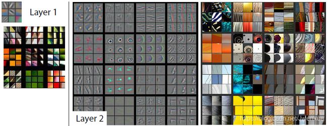
While visualization of a trained model gives insight into its operation, it can also assist with selecting good architectures in the first place. By visualizing the first and second layers of Krizhevsky et al. ’s architecture (Fig. 5(a) & (c)), various problems are apparent. The first layer filters are a mix of extremely high and low frequency information, with little coverage of the mid frequencies. Additionally, the 2nd layer visualization shows aliasing artifacts caused by the large stride 4 used in the 1st layer convolutions. To remedy these problems, we (i) reduced the 1st layer filter size from 11x11 to 7x7 and (ii) made the stride of the convolution 2, rather than 4. This new architecture retains much more information in the 1st and 2nd layer features, as shown in Fig. 5(b) & (d). More importantly, it also improves the classification performance as shown in Section 5.1.

4.1 框架选择

虽然训练模型的可视化可以深入了解其操作，但它也可以帮助您首选好的架构。通过可视化Krizhevsky等架构（图5（a）和（c））的第一层和第二层，各种问题都很明显。第一层滤波器是极高和极低频信息的混合，几乎没有涵盖中频信息。另外，第二层可视化呈现出由第一层卷积中使用的大步幅4引起的混叠伪影。为了解决这些问题，我们（i）将第一层滤波器尺寸从11x11缩小到7x7，并且（ii）使卷积的步幅由4改为2。如图5（b）和（d）所示，这种新架构在第1层和第2层特征中保留了更多信息。更重要的是，如第5.1节所示，它还提高了分类性能。

4.2 Occlusion Sensitivity

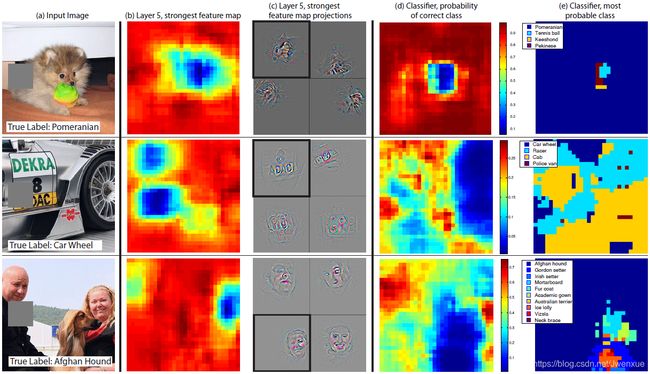
With image classification approaches, a natural question is if the model is truly identifying the location of the object in the image, or just using the surrounding context. Fig. 6 attempts to answer this question by systematically occluding different portions of the input image with a grey square, and monitoring the output of the classifier. The examples clearly show the model is localizing the objects within the scene, as the probability of the correct class drops significantly when the object is occluded. Fig. 6 also shows visualizations from the strongest feature map of the top convolution layer, in addition to activity in this map (summed over spatial locations) as a function of occluder position. When the occluder covers the image region that appears in the visualization, we see a strong drop in activity in the feature map. This shows that the visualization genuinely corresponds to the image structure that stimulates that feature map, hence validating the other visualizations shown in Fig. 4 and Fig. 2.

Fig. 4. Evolution of a randomly chosen subset of model features through training. Each layer’s features are displayed in a different block. Within each block, we show a randomly chosen subset of features at epochs [1,2,5,10,20,30,40,64]. The visualization shows the strongest activation (across all training examples) for a given feature map, projected down to pixel space using our deconvnet approach. Color contrast is artificially enhanced and the figure is best viewed in electronic form.

Fig. 5. (a): 1st layer features without feature scale clipping. Note that one feature dominates. (b): 1st layer features from Krizhevsky et al. [18]. (c): Our 1st layer features. The smaller stride (2 vs 4) and filter size (7x7 vs 11x11) results in more distinctive features and fewer “dead” features. (d): Visualizations of 2nd layer features from Krizhevsky et al. [18]. (e): Visualizations of our 2nd layer features. These are cleaner, with no aliasing artifacts that are visible in (d).

Fig. 6. Three test examples where we systematically cover up different portions of the scene with a gray square (1st column) and see how the top (layer 5) feature maps ((b) & (c)) and classifier output ((d) & (e)) changes. (b): for each position of the gray scale, we record the total activation in one layer 5 feature map (the one with the strongest response in the unoccluded image). (c): a visualization of this feature map projected down into the input image (black square), along with visualizations of this map from other images. The first row example shows the strongest feature to be the dog’s face. When this is covered-up the activity in the feature map decreases (blue area in (b)). (d): a map of correct class probability, as a function of the position of the gray square. E.g. when the dog’s face is obscured, the probability for “pomeranian” drops significantly. (e): the most probable label as a function of occluder position. E.g. in the 1st row, for most locations it is “pomeranian”, but if the dog’s face is obscured but not the ball, then it predicts “tennis ball”. In the 2nd example, text on the car is the strongest feature in layer 5, but the classifier is most sensitive to the wheel. The 3rd example contains multiple objects. The strongest feature in layer 5 picks out the faces, but the classifier is sensitive to the dog (blue region in (d)), since it uses multiple feature maps.

Fig. 7. Caltech-256 classification performance as the number of training images per class is varied. Using only 6 training examples per class with our pre-trained feature extractor, we surpass best reported result by Bo et al. [3].

4.2 遮挡敏感度

使用图像分类方法，一个自然的问题是模型是否真正识别图像中对象的位置，或者只是使用周围的上下文信息。图6试图通过用灰色方块系统地遮挡输入图像的不同部分并观察分类器的输出，以此尝试解决这个问题。这些示例清楚地表明模型能够定位场景中的对象，尽管当对象被遮挡时正确类的概率会显着下降。图6还示出了来自顶部卷积层的最强特征图的可视化，以及该特征图中的激活（在空间位置上求和）作为遮挡物位置的函数。当遮挡物覆盖可视化中出现的图像区域时，我们会看到特征图中激活的明显下降。这表明可视化真实地对应于激活该特征图的图像结构，图4和图2所示为验证了其他可视化。

图4.通过训练随机选择的模型特征子集的演变。每个图层的特征都显示在不同的块中。在每个块内，我们在epoch[1,2,5,10,20,30,40,64]随机选择特征子集。可视化显示给定特征图的最强激活（在所有训练示例中），使用我们的反卷积方法向下投影到像素空间。人工增强色彩对比度，最好以电子形式观看。

图5.（a）：第一层特征没有特征尺度削减。请注意，一个特征占主导地位。（b）：Krizhevsky等[18]的第一层特征。（c）：我们的第一层特征。较小的步长（2 vs 4）和卷积核尺寸（7x7 vs 11x11）导致更多特色和更少的“死”特征。（d）：Krizhevsky等[18]的第二层特征的可视化。（e）：我们的第二层特征的可视化。它们更干净，没有（d）中可见的混叠伪影。

图6.三个测试示例，我们系统地用灰色方块（第1列）覆盖场景的不同部分，并查看顶部（第5层）特征如何映射（（b）和（c））和分类器输出（（d）＆（e））如何变化。（b）：对于灰度区域的每个位置，我们在一个第5层特征图（在未被遮挡的图像中具有最强响应的那个）中记录总激活。（c）：向下投影到输入图像（黑色方块）中的此特征地图的可视化，以及来自其他图像的该地图的可视化。第一行示例显示了最强的特征是狗的脸。当掩盖它时，特征图中的激活降低（（b）中的蓝色区域）。（d）：正确类概率的映射，作为灰色方块位置的函数。例如。当狗的脸被遮挡时，“博美犬”的概率显着下降。（e）：最可能的标签作为遮挡位置的函数。例如。在第1排，对于大多数位置，它是“博美犬”，但如果狗的脸被遮挡而不是球，那么它预测“网球”。在第二个示例中，汽车上的文本是第5层中最强的特征，但分类器对车轮最敏感。第3个示例包含多个对象。第5层中最强的特征是挑选出了面部，但是分类器对狗敏感（（d）中的蓝色区域），因为它使用多个特征映射。

图7. Caltech-256分类性能随着每个类别训练图像数量的变化而变化。使用每个类别仅用6个训练样例预训练的特征提取器，其结果超过Bo等[3]的最佳报告结果。

5 Experiments

5. 实验

5.1 ImageNet 2012

This dataset consists of 1.3M/50k/100k training/validation/test examples, spread over 1000 categories. Table 1 shows our results on this dataset.

Table 1. ImageNet 2012/2013 classification error rates. The ∗ indicates models that were trained on both ImageNet 2011 and 2012 training sets.

5.1 ImageNet 2012

该数据集由1.3M/50k/100k训练/验证/测试样例组成，分布在1000个类别中。表1显示了我们在此数据集上的结果。

表1. ImageNet 2012/2013分类错误率。*表示在ImageNet 2011和2012训练集上都经过训练的模型。

Using the exact architecture specified in Krizhevsky et al. [18], we attempt to replicate their result on the validation set. We achieve an error rate within 0.1% of their reported value on the ImageNet 2012 validation set.

使用Krizhevsky等[18]指出的确切架构，我们尝试在验证集上复现他们的结果。我们达到了他们在ImageNet 2012验证集上报告的0.1％的错误率。

Next we analyze the performance of our model with the architectural changes outlined in Section 4.1 (7×7 filters in layer 1 and stride 2 convolutions in layers 1 & 2). This model, shown in Fig. 3, significantly outperforms the architecture of Krizhevsky et al. [18], beating their single model result by 1.7% (test top-5). When we combine multiple models, we obtain a test error of 14.8%, an improvement of 1.6%. This result is close to that produced by the data-augmentation approaches of Howard [15], which could easily be combined with our architecture. However, our model is some way short of the winner of the 2013 Imagenet classification competition [28].

Fig. 3. Architecture of our 8 layer convnet model. A 224 by 224 crop of an image (with 3 color planes) is presented as the input. This is convolved with 96 different 1st layer filters (red), each of size 7 by 7, using a stride of 2 in both x and y. The resulting feature maps are then: (i) passed through a rectified linear function (not shown), (ii) pooled (max within 3x3 regions, using stride 2) and (iii) contrast normalized across feature maps to give 96 different 55 by 55 element feature maps. Similar operations are repeated in layers 2,3,4,5. The last two layers are fully connected, taking features from the top convolutional layer as input in vector form (6·6·256 = 9216 dimensions). The final layer is a C-way softmax function, C being the number of classes. All filters and feature maps are square in shape.

接下来，我们分析了第4.1节（第1层中的7×7过滤器和第1层和第2层中的步长为2的卷积）中概述的改变框架的模型的性能。如图3所示，该模型明显优于Krizhevsky等[18]的架构，击败了他们单一模型1.7％（测试top-5）的结果。当我们组合多个模型时，我们获得了14.8％的测试误差，提高了1.6％。这个结果接近于Howard [15]通过数据增强所产生的结果，这个架构可以很容易地与我们的架构相结合。然而，我们的模型比2013年Imagenet分类竞赛的获胜的模型[28]短小。

图3.我们8层卷积模型的架构。图像（具有3个颜色通道）224×224大小的裁剪作为输入。用96个不同的第一层滤波器（红色）对其进行卷积，每个滤波器的尺寸为7×7，步长为2。然后得到的特征图：（i）通过整流的线性函数（图中未显示），（ii）池化（在3×3区域内取最大值，步长为2）和（iii）在特征图上进行对比度标准化，得到96个不同的55×55个元素特征映射。在2,3,4,5层中重复类似的操作。最后两层为全连接，将顶部卷积层的特征以向量形式（6·6·256=9216维）作为其输入。最后一层是C个类别的softmax函数，C是类别的数量。所有卷积核和特征图都是方形的。

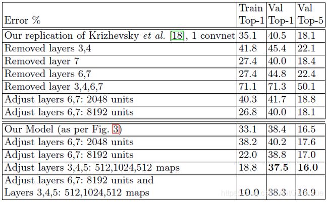
Varying ImageNet Model Sizes: In Table 2, we first explore the architecture of Krizhevsky et al. [18] by adjusting the size of layers, or removing them entirely. In each case, the model is trained from scratch with the revised architecture. Removing the fully connected layers (6,7) only gives a slight increase in error (in the following, we refer to top-5 validation error). This is surprising, given that they contain the majority of model parameters. Removing two of the middle convolutional layers also makes a relatively small difference to the error rate. However, removing both the middle convolution layers and the fully connected layers yields a model with only 4 layers whose performance is dramatically worse. This would suggest that the overall depth of the model is important for obtaining good performance. We then modify our model, shown in Fig. 3. Changing the size of the fully connected layers makes little difference to performance (same for model of Krizhevsky et al. [18]). However, increasing the size of the middle convolution layers goes give a useful gain in performance. But increasing these, while also enlarging the fully connected layers results in over-fitting.

Table 2. ImageNet 2012 classification error rates with various architectural changes to the model of Krizhevsky et al. [18] and our model (see Fig. 3)

改变ImageNet模型尺寸：在表2中，我们首先通过调整图层的大小，或完全删除的方式探索了Krizhevsky等[18]的架构。在每种情况下，修改架构后的模型都是从头开始训练。删除全连接层（6,7层）只会略微增加错误率（在下文中，指的是top-5验证错误率）。这是令人惊讶的，因为这两层包含大多数的模型参数。移除两个中间卷积层也会对错误率产生相对较小的差异。然而，同时去除中间卷积层和全连接层而产生仅具有4层的模型，其性能显著变差。这可能表明模型的整体深度对于获得良好的性能至关重要。之后，如图3所示，修改我们的模型。改变全连接层的大小对性能几乎没有影响（Krizhevsky等[18]模型也是如此）。但是，增加中间卷积层的大小可以提高性能。但增加这些，将会同时增大全连接层，从而会导致过拟合。

表2.对Krizhevsky等[18]模型和我们的模型（见图3）经过不同改变的模型在ImageNet 2012上的分类错误率

5.2 Feature Generalization

The experiments above show the importance of the convolutional part of our ImageNet model in obtaining state-of-the-art performance. This is supported by the visualizations of Fig. 2 which show the complex invariances learned in the convolutional layers. We now explore the ability of these feature extraction layers to generalize to other datasets, namely Caltech-101 [9], Caltech-256 [11] and PASCAL VOC 2012. To do this, we keep layers 1-7 of our ImageNet-trained model fixed and train a new softmax classifier on top (for the appropriate number of classes) using the training images of the new dataset. Since the softmax contains relatively few parameters, it can be trained quickly from a relatively small number of examples, as is the case for certain datasets.

5.2 特征泛化

上面的实验表明了我们ImageNet模型的卷积部分在获得最先进性能方面的重要性。这由图2的可视化可以佐证，其显示了卷积层中学习到的复杂不变性。我们现在探索这些特征提取层泛化到其他数据集的能力，即Caltech-101 [9]，Caltech-256 [11]和PASCAL VOC 2012.为此，我们保持ImageNet训练的模型1-7层固定，并且在模型顶端使用新数据集的训练数据训练一个新的softmax分类器（类别数量）。由于softmax包含相对较少的参数，因此可以从相对少量的样例中快速训练，如某些数据集的情况。

The experiments compare our feature representation, obtained from ImageNet, with the hand-crafted features used by other methods. In both our approach and existing ones the Caltech/PASCAL training data is only used to train the classifier. As they are of similar complexity (ours: softmax, others: linear SVM), the feature representation is crucial to performance. It is important to note that both representations were built using images beyond the Caltech and PASCAL training sets. For example, the hyper-parameters in HOG descriptors were determined through systematic experiments on a pedestrian dataset [5].

实验将我们从ImageNet获得的特征表示与其他方法使用的手工制作的特征进行了比较。在我们的方法和现有方法中，Caltech/PASCAL训练数据仅用于训练分类器。由于这些方法具有相似的复杂性（我们的模型：softmax，其他模型：线性SVM），因此特征表示对性能至关重要。值得注意的是，两种表示都是使用Caltech和PASCAL训练集之外的图像构建的。例如，HOG模型中的超参数是通过对行人数据集的系统实验来确定的[5]。

We also try a second strategy of training a model from scratch, i.e. resetting layers 1-7 to random values and train them, as well as the softmax, on the training images of the PASCAL/Caltech dataset.

我们还尝试了从头开始训练模型的第二种策略，即将1-7层重置为随机值，并与softmax一同在PASCAL / Caltech数据集的训练图像上进行训练。

One complication is that some of the Caltech datasets have some images that are also in the ImageNet training data. Using normalized correlation, we identified these few “overlap” images2 and removed them from our Imagenet training set and then retrained our Imagenet models, so avoiding the possibility of train/test contamination.

一个复杂的问题是，一些Caltech数据集中的图像也存在于ImageNet训练数据中。使用归一化相关性，我们识别出这些“重复”图像2，并将它们从我们的Imagenet训练集中移除，然后重新训练我们的Imagenet模型，从而避免了训练/测试污染的可能性。

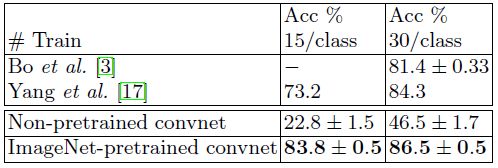
Caltech-101: We follow the procedure of [9] and randomly select 15 or 30 images per class for training and test on up to 50 images per class reporting the average of the per-class accuracies in Table 3, using 5 train/test folds. Training took 17 minutes for 30 images/class. The pre-trained model beats the best reported result for 30 images/class from [3] by 2.2%. Our result agrees with the recently published result of Donahue et al. [7], who obtain 86.1% accuracy (30 imgs/class). The convnet model trained from scratch however does terribly, only achieving 46.5%, showing the impossibility of training a large convnet on such a small dataset.

Table 3. Caltech-101 classification accuracy for our convnet models, against two leading alternate approaches

Caltech-101：我们按照[9]的步骤，使用5倍的训练/测试拆分，每个类别随机选择15或30张图像进行训练，并且每个类别测试最多50张图像，表3报告了每类准确度平均值。30张图像/类别的训练需要17分钟。预训练模型通过2.2％的结果击败了来自[3]的30图像/类别的最佳报告结果。我们的结果与最近公布的Donahue等[7]的86.1％的准确率（30图像/类别）结果一致。然而，从头开始训练的卷积网模型确实非常糟糕，只达到了46.5％，表明在如此小的数据集上训练大型卷积网络比较不可行。

表3.我们的卷积网络模型与两种领先的类似方法在Caltech-101上的分类准确度比较

Caltech-256: We follow the procedure of [11], selecting 15, 30, 45, or 60 training images per class, reporting the average of the per-class accuracies in Table 4. Our ImageNet-pretrained model beats the current state-of-the-art results obtained by Bo et al. [3] by a significant margin: 74.2% vs 55.2% for 60 training images/class. However, as with Caltech-101, the model trained from scratch does poorly. In Fig. 7, we explore the “one-shot learning” [9] regime. With our pretrained model, just 6 Caltech-256 training images are needed to beat the leading method using 10 times as many images. This shows the power of the ImageNet feature extractor.

Table 4. Caltech 256 classification accuracies

Caltech-256：我们按照[11]的步骤，每个类别选择15,30,45或60张训练图像，表4报告了中每个类别准确度平均值。我们的ImageNet预训练模型远远胜过Bo等[3]取得的目前最好的结果：60训练图像/类别准确率相比为74.2％ vs 55.2％。然而，与Caltech-101一样，从头开始训练的模型也很差。在图7中，我们探索了“一次性学习”[9]方式。使用我们的预训练的模型，只需要6张Caltech-256训练图像就可以击败使用10倍之多图像的领先方法。这显示了ImageNet特征提取器的强大功能。

表4. Caltech 256分类准确率

PASCAL 2012: We used the standard training and validation images to train a 20-way softmax on top of the ImageNet-pretrained convnet. This is not ideal, as PASCAL images can contain multiple objects and our model just provides a single exclusive prediction for each image. Table 5 shows the results on the test set, comparing to the leading methods: the top 2 entries in the competition and concurrent work from Oquab et al. [21] who use a convnet with a more appropriate classifier. The PASCAL and ImageNet images are quite different in nature, the former being full scenes unlike the latter. This may explain our mean performance being 3.2% lower than the leading competition result [27], however we do beat them on 5 classes, sometimes by large margins.

Table 5. PASCAL 2012 classification results, comparing our Imagenet-pretrained convent against the leading two methods and the recent approach of Oquab et al. [21]

PASCAL 2012：我们使用标准的训练和验证图像在ImageNet预训练的卷积网络上训练20个类别的softmax。这并不理想，因为PASCAL图像可能包含多个对象，而我们的模型为每个图像只提供独一无二的预测结果。表5显示了测试集上的结果，并与领先方法进行相比：竞赛中的前2名和Oquab等[21]的同期研究，其使用一个更合适分类器的卷积网络。PASCAL和ImageNet图像在本质上是完全不同的，前者是完整的场景，而后者不是。这可以解释我们的平均性能比领先的竞赛者[27]结果低27％，但是我们确实在5分类的任务上击败它们，有时候是完胜。

表5. PASCAL 2012分类结果，我们的Imagenet预训练卷积网络与领先的两种方法和Oquab等[21]近期的方法进行比较

5.3 Feature Analysis

We explore how discriminative the features in each layer of our Imagenet-pretrained model are. We do this by varying the number of layers retained from the ImageNet model and place either a linear SVM or softmax classifier on top. Table 6 shows results on Caltech-101 and Caltech-256. For both datasets, a steady improvement can be seen as we ascend the model, with best results being obtained by using all layers. This supports the premise that as the feature hierarchies become deeper, they learn increasingly powerful features.

Table 6. Analysis of the discriminative information contained in each layer of feature maps within our ImageNet-pretrained convnet. We train either a linear SVM or softmax on features from different layers (as indicated in brackets) from the convnet. Higher layers generally produce more discriminative features.

5.3特征分析

我们探讨了Imagenet预训练模型的每一层是如何区别特征的。我们通过改变从ImageNet模型重新训练的网络层数，并在顶部放置线性SVM或softmax分类器来实现此目的。表6显示了在Caltech-101和Caltech-256数据集上的结果。对于这两个数据集，当我们提升模型时可以看到效果稳定的改进，通过使用所有层获得最佳结果。这支持了这样一个前提：当特征层次结构变得更深时，它们会学习到越来越强大的特征。

表6.我们ImageNet预训练卷积网络中每层特征映射中包含判别信息的分析。我们对卷积网络不同层（如括号中所示）的特征上训练线性SVM或softmax分类器。较高层通常产生更多的辨别特征。

6 Discussion

We explored large convolutional neural network models, trained for image classification, in a number ways. First, we presented a novel way to visualize the activity within the model. This reveals the features to be far from random, uninterpretable patterns. Rather, they show many intuitively desirable properties such as compositionality, increasing invariance and class discrimination as we ascend the layers. We also show how these visualization can be used to identify problems with the model and so obtain better results, for example improving on Krizhevsky et al. ’s [18] impressive ImageNet 2012 result. We then demonstrated through a series of occlusion experiments that the model, while trained for classification, is highly sensitive to local structure in the image and is not just using broad scene context. An ablation study on the model revealed that having a minimum depth to the network, rather than any individual section, is vital to the model’s performance.

6讨论

我们以多种方式探索了这些通过图像分类训练到的大型卷积神经网络模型。首先，我们提出了一种可视化模型中激活的新方法。这表明这些特征并非随机，而是无法解释的模式。相反，当我们提升层次时，它们显示出许多直观上令人满意的属性，例如组合性，增加不变性和类别区分度。我们还展示了如何使用这些可视化来识别模型的问题，从而获得更好的结果，例如改进Krizhevsky等[18]的令人印象深刻的ImageNet 2012结果。然后，我们通过一系列遮挡实验证明，该模型虽然经过分类训练，但对图像中的局部结构非常敏感，并且不仅仅使用广泛的场景环境。对该模型的消融研究表明，对网络而言，最小深度对模型的性能至关重要，而不是其它任何单个部分，。

Finally, we showed how the ImageNet trained model can generalize well to other datasets. For Caltech-101 and Caltech-256, the datasets are similar enough that we can beat the best reported results, in the latter case by a significant margin. Our convnet model generalized less well to the PASCAL data, perhaps suffering from dataset bias [25], although it was still within 3.2% of the best reported result, despite no tuning for the task. For example, our performance might improve if a different loss function was used that permitted multiple objects per image. This would naturally enable the networks to tackle the object detection as well.

最后，我们展示了ImageNet训练模型如何能够很好地泛化到其他数据集。对于Caltech-101和Caltech-256，数据集足够相似，我们击败了报告的最佳结果，在后一个数据集上以显著的优势获胜。我们的卷积模型不太适用于PASCAL数据，可能是因为存在数据集偏差[25]，尽管在没有对任务进行调整的情况下它仍然在最佳报告结果的3.2％之内。例如，如果使用允许每个图像有多个对象的不同损失函数，我们的性能可能会提高。这自然会使网络也能够解决对象检测问题。

Acknowledgments

The authors would like to thank Yann LeCun for helpful discussions and acknowledge support from NSERC, NSF grant #1116923 and Microsoft Research.

致谢

作者们感谢Yann LeCun的富有帮助的讨论，感谢NSERC，NSF＃1116923资助和微软研究院的支持。

References

参考文献

1. Bengio, Y., Lamblin, P., Popovici, D., Larochelle, H.: Greedy layer-wise training of deep networks. In: NIPS, pp. 153–160 (2007)

2. Berkes, P., Wiskott, L.: On the analysis and interpretation of inhomogeneous quadratic forms as receptive fields. Neural Computation (2006)

3. Bo, L., Ren, X., Fox, D.: Multipath sparse coding using hierarchical matching pursuit. In: CVPR (2013)

4. Ciresan, D.C., Meier, J., Schmidhuber, J.: Multi-column deep neural networks for image classification. In: CVPR (2012)

5. Dalal, N., Triggs, B.: Histograms of oriented gradients for pedestrian detection. In: CVPR (2005)

6. Deng, J., Dong, W., Socher, R., Li, L.J., Li, K., Fei-Fei, L.: ImageNet: A Large-Scale Hierarchical Image Database. In: CVPR 2009 (2009)

7. Donahue, J., Jia, Y., Vinyals, O., Hoffman, J., Zhang, N., Tzeng, E., Darrell, T.: DeCAF: A deep convolutional activation feature for generic visual recognition. arXiv:1310.1531 (2013)

8. Erhan, D., Bengio, Y., Courville, A., Vincent, P.: Visualizing higher-layer features of a deep network. Technical report, University of Montreal (2009)

9. Fei-fei, L., Fergus, R., Perona, P.: One-shot learning of object categories. IEEE Trans. PAMI (2006)

10. Girshick, R., Donahue, J., Darrell, T., Malik, J.: Rich feature hierarchies for accurate object detection and semantic segmentation. arXiv:1311.2524 (2014)

11. Griffin, G., Holub, A., Perona, P.: The caltech 256. Caltech Technical Report (2006)

12. Gunji, N., Higuchi, T., Yasumoto, K., Muraoka, H., Ushiku, Y., Harada, T., Kuniyoshi, Y.: Classification entry. Imagenet Competition (2012)

13. Hinton, G.E., Osindero, S., Teh, Y.: A fast learning algorithm for deep belief nets. Neural Computation 18, 1527–1554 (2006)

14. Hinton, G.E., Srivastave, N., Krizhevsky, A., Sutskever, I., Salakhutdinov, R.R.: Improving neural networks by preventing co-adaptation of feature detectors. In: arXiv:1207.0580 (2012)

15. Howard, A.G.: Some improvements on deep convolutional neural network based image classification. arXiv 1312.5402 (2013)

16. Jarrett, K., Kavukcuoglu, K., Ranzato, M., LeCun, Y.:What is the best multi-stage architecture for object recognition? In: ICCV (2009)

17. Jianchao, Y., Kai, Y., Yihong, G., Thomas, H.: Linear spatial pyramid matching using sparse coding for image classification. In: CVPR (2009) Visualizing and Understanding Convolutional Networks 833

18. Krizhevsky, A., Sutskever, I., Hinton, G.: Imagenet classification with deep convolutional neural networks. In: NIPS (2012)

19. Le, Q.V., Ngiam, J., Chen, Z., Chia, D., Koh, P., Ng, A.Y.: Tiled convolutional neural networks. In: NIPS (2010)

20. LeCun, Y., Boser, B., Denker, J.S., Henderson, D., Howard, R.E., Hubbard, W., Jackel, L.D.: Backpropagation applied to handwritten zip code recognition. Neural Comput. 1(4), 541–551 (1989)

21. Oquab, M., Bottou, L., Laptev, I., Sivic, J.: Learning and transferring mid-level image representations using convolutional neural networks. In: CVPR (2014)

22. Sande, K., Uijlings, J., Snoek, C., Smeulders, A.: Hybrid coding for selective search. In: PASCAL VOC Classification Challenge 2012 (2012)

23. Simonyan, K., Vedaldi, A., Zisserman, A.: Deep inside convolutional networks: Visualising image classification models and saliency maps. arXiv 1312.6034v1 (2013)

24. Sohn, K., Jung, D., Lee, H., Hero III, A.: Efficient learning of sparse, distributed, convolutional feature representations for object recognition. In: ICCV (2011)

25. Torralba, A., Efros, A.A.: Unbiased look at dataset bias. In: CVPR (2011)

26. Vincent, P., Larochelle, H., Bengio, Y., Manzagol, P.A.: Extracting and composing robust features with denoising autoencoders. In: ICML, pp. 1096–1103 (2008)

27. Yan, S., Dong, J., Chen, Q., Song, Z., Pan, Y., Xia, W., Huang, Z., Hua, Y., Shen, S.: Generalized hierarchical matching for sub-category aware object classification. In: PASCAL VOC Classification Challenge 2012 (2012)

28. Zeiler, M.: Clarifai (2013), http://www.image-net.org/challenges/LSVRC/2013/ results.php

29. Zeiler, M., Taylor, G., Fergus, R.: Adaptive deconvolutional networks for mid and high level feature learning. In: ICCV (2011)