sklearn中的metrics

多分类的metrix问题，请见多分类问题。

MSE

我们先看一下回归问题常用的均方根误差MSE。

from sklearn.metrics import mean_squared_error
housing_pred = lin_reg.predict(housing_feature)
lin_mse = mean_squared_error(housing_label, housing_pred)
print(np.sqrt(lin_mse))

69658.1903557702

交叉验证

使用sklearn提供的cross_val_score()，我们可以很方便的交叉验证模型效果。比如，我们看一下上面5和非5的线性分类器的准确率：

from sklearn.model_selection import cross_val_score, cross_val_predict
cross_val_score(sgd_clf, X_train, y_train_5, cv=3, scoring='accuracy')

array([0.9615, 0.9595, 0.9535])

上述代码中，我们随机划分训练数据和测试数据，训练模型后计算准确率，并重复了3次。

准确率、精度、召回率、F1、AUC

下面我们主要看一下准确率、精度、召回率、F1、ROC/AUC等常用于二分类问题的metrics。

准确率

from sklearn.metrics import accuracy_score, confusion_matrix, precision_score, recall_score, f1_score, precision_recall_curve
y_pred_5 = sgd_clf.predict(X_test)

accuracy_score(y_test_5, y_pred_5)

0.96165625

混淆矩阵

confusion_matrix(y_test_5, y_pred_5)

array([[57323,   878],
       [ 1576,  4223]])

精度、召回率、F1

precision_score(y_test_5, y_pred_5)

0.8278768868849246

recall_score(y_test_5, y_pred_5)

0.7282290050008622

f1_score(y_test_5, y_pred_5)

0.774862385321101

ROC & AUC

from sklearn.metrics import roc_auc_score
roc_auc_score(y_test_5, y_pred_5)

0.856571676775787

阈值衡量、ROC曲线

sklearn不允许对分类模型直接设置阈值，但是可以访问它用于预测的决策分数。不是调用分类器的predict()函数，而是调用decision_function()函数，这种方法返回每个实例的分数，然后就可以根据这些分数，使用任意阈值进行预测了。

我们先看个示例：

y_pred = sgd_clf.predict([X_test[11]])
print(y_pred)

y_score = sgd_clf.decision_function([X_test[11]])
print(y_score)

[ True]
[58446.52780903]

我们随机抽取了一个样本，其score=41983，而默认的阈值为0，所以预测结果为True。如果我们现在想提高精度（降低其召回率），那可以提高其阈值：

threshold = 50000
y_predict_t = (y_score > threshold)
print(y_predict_t)

accuracy = accuracy_score(y_test, y_predict_t)
precision = precision_score(y_test, y_predict_t)
recall = recall_score(y_test, y_predict_t)
f1 = f1_score(y_test, y_predict_t)
auc = roc_auc_score(y_test, y_predict_t)
print(accuracy, precision, recall, f1, auc)

[ True]

阈值选择

那怎么选取合适的阈值呢？

我们先使用cross_val_predict()获取决策分数而非预测结果；然后使用precision_recall_curve()计算所有可能阈值的精度和召回率；最后使用matplotlib绘制精度和召回率相对于阈值的函数组：

y_score = cross_val_predict(sgd_clf, X_train, y_train_5, cv=3, method='decision_function')
precisions, recalls, thresholds = precision_recall_curve(y_train_5, y_score)
def plot_precision_recall_vs_threshold(precisions, recalls, thresholds):
    plt.plot(thresholds, precisions[:-1], 'b--', label='Precision')
    plt.plot(thresholds, recalls[:-1], 'g-', label='Recall')
    
plot_precision_recall_vs_threshold(precisions, recalls, thresholds)
plt.show()

根据上图，可以选择合适的阈值。

假设你决定将精度设置为90%：

threshold_90_precision = thresholds[np.argmax(precisions>=0.90)]
print(threshold_90_precision)

261289.38745837728

取的合适的阈值后，我们可以这样指定最终的预测结果：

y_pred_90 = (y_score >= threshold_90_precision)
print(y_pred_90)

[False False False ... False False False]

ROC曲线

画ROC曲线和上述的精度、召回率曲线类似，但要先算出FPR和TPR：

from sklearn.metrics import roc_curve
fpr, tpr, thresholds = roc_curve(y_train_5, y_score)
def plt_roc_curve(fpr, tpr, label=None):
    plt.plot(fpr, tpr, linewidth=2, label=label)
    plt.plot([0,1], [0,1], 'k--')
    
plt_roc_curve(fpr, tpr)
plt.show()

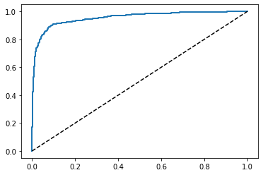
画出ROC曲线后，可用上述的方法计算得到AUC：

roc_auc_score(y_test_5, y_pred_5)

0.856571676775787