卷积神经网络经典论文的学习笔记
- 1 Optimization algorithm And Regularization
- 1.1 Optimization algorithm
- 1.2 Regularization
- 2 Convolutional Neural Network
- 2.1 Convolution
- General development process
- 2.2 Deconvolution
- 2.3 Classical convolution networks
- 2.3.1 AlexNet- ImageNet Classification with Deep Convolutional Neural Networks
- 2.3.2 VGG- VERY DEEP CONVOLUTIONAL NETWORKS FOR LARGE-SCALE IMAGE RECOGNITION
- 2.3.3 NIN- Network in Network
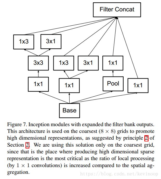
- 2.3.4 Inception V3
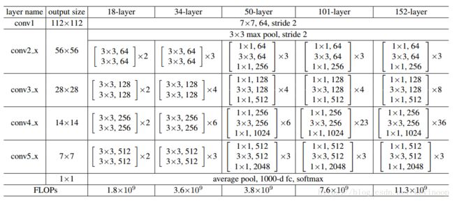
- 2.3.5 ResNet- Deep Residual Learning for Image Recognition
- 2.1 Convolution
- 3 Neural Style Transfer
- 3.1 A Neural Algorithm of Artistic Style(L. A. Gatys)
- 4 Autoencoder
- 4.1 Stacked Denoising Autoencoders: Learning Useful Representations …
1 Optimization algorithm And Regularization
1.1 Optimization algorithm
GD(SGD、MBGD、BGD)
SGDM (Momentum)
Vdω=β∗Vdω+(1−β)∗dω V d ω = β ∗ V d ω + ( 1 − β ) ∗ d ω
Vdb=β∗Vdb+(1−β)∗db V d b = β ∗ V d b + ( 1 − β ) ∗ d b
ω:=ω−α∗Vdω ω := ω − α ∗ V d ω
b:=b−α∗Vdb b := b − α ∗ V d b
( β=0.9 β = 0.9 )
RMSPROP
Sdw=β∗Sdw+(1−β)∗(dω)2 S d w = β ∗ S d w + ( 1 − β ) ∗ ( d ω ) 2
Sdb=β∗Sdb+(1−β)∗(db)2 S d b = β ∗ S d b + ( 1 − β ) ∗ ( d b ) 2
ω:=ω−α∗dωSdw√+ϵ ω := ω − α ∗ d ω S d w + ϵ
b:=b−α∗dbSb√+ϵ b := b − α ∗ d b S b + ϵ
( ϵ=10−8 ϵ = 10 − 8 )
Adam
Vdω=β1∗Vdω+(1−β1)∗dω V d ω = β 1 ∗ V d ω + ( 1 − β 1 ) ∗ d ω
Vdb=β1∗Vdb+(1−β1)∗db V d b = β 1 ∗ V d b + ( 1 − β 1 ) ∗ d b
Sdw=β2∗Sdw+(1−β2)∗(dω)2 S d w = β 2 ∗ S d w + ( 1 − β 2 ) ∗ ( d ω ) 2
Sdb=β2∗Sdb+(1−β2)∗(db)2 S d b = β 2 ∗ S d b + ( 1 − β 2 ) ∗ ( d b ) 2
Vcorrectdω=Vdω1−βt1 V d ω c o r r e c t = V d ω 1 − β 1 t Vcorrectdb=Vdb1−βt1 V d b c o r r e c t = V d b 1 − β 1 t
Scorrectdω=Sdω1−βt2 S d ω c o r r e c t = S d ω 1 − β 2 t Scorrectdb=Sdb1−βt2 S d b c o r r e c t = S d b 1 − β 2 t
ω:=ω−α∗VcorrectdωScorrectdω√+ϵ ω := ω − α ∗ V d ω c o r r e c t S d ω c o r r e c t + ϵ
b:=b−α∗VcorrectdbScorrectb√+ϵ b := b − α ∗ V d b c o r r e c t S b c o r r e c t + ϵ( β1=0.9β2=0.99ϵ=10−8 β 1 = 0.9 β 2 = 0.99 ϵ = 10 − 8 )
1.2 Regularization
Batch Norm
μ=1m∗∑izi μ = 1 m ∗ ∑ i z i
σ2=1m∗∑i(zi−μ)2 σ 2 = 1 m ∗ ∑ i ( z i − μ ) 2
zinorm=zi−μσ2+ϵ√ z n o r m i = z i − μ σ 2 + ϵ
z^inorm=γ∗zinorm+β z ^ n o r m i = γ ∗ z n o r m i + β
( γ and β γ a n d β are used to adjust the expectation and variance)
Dropout
keep_prob=0.8
d3 = np.random.rand( a3.shape[0],a3.shape[1]) < keep_prob # activate 80%
a3 =np.multiply(a3,d3)
a3/=keep_prob #使激活值期望不变
2 Convolutional Neural Network
2.1 Convolution
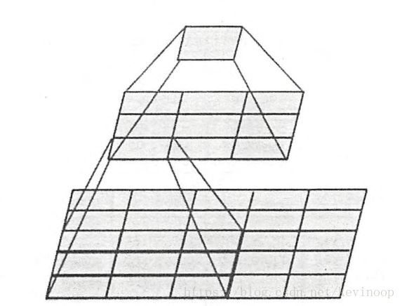
Convolution
f[l]=filter sizep[l]=paddings[l]=stride f [ l ] = f i l t e r s i z e p [ l ] = p a d d i n g s [ l ] = s t r i d e
Input: n[l−1]H∗n[l−1]w∗n[l−1]c n H [ l − 1 ] ∗ n w [ l − 1 ] ∗ n c [ l − 1 ] (height& width& channel)
Output: n[l]H∗n[l]w∗n[l]c n H [ l ] ∗ n w [ l ] ∗ n c [ l ]
n[l]H=⌊n[l−1]H+2p[l]−f[l]s[l]+1⌋ n H [ l ] = ⌊ n H [ l − 1 ] + 2 p [ l ] − f [ l ] s [ l ] + 1 ⌋
n[l]w=⌊n[l−1]w+2p[l]−f[l]s[l]+1⌋ n w [ l ] = ⌊ n w [ l − 1 ] + 2 p [ l ] − f [ l ] s [ l ] + 1 ⌋
if Padding=’VALID’ ,then output is to be : n=⌊n[l−1]w−f[l]s[l]+1⌋ n = ⌊ n w [ l − 1 ] − f [ l ] s [ l ] + 1 ⌋
if Padding=’SAME’ ,then output is to be :
Sparse connection & Weight sharing
Pooling
f f : filter sizes s : stride
nH=⌊nH−fs+1⌋ n H = ⌊ n H − f s + 1 ⌋
nw=⌊nw−fs+1⌋ n w = ⌊ n w − f s + 1 ⌋
Fully connected
General development process
2.2 Deconvolution
Convolution process:
input: 4∗4 4 ∗ 4 filter: 3∗3 3 ∗ 3 (s=1,p=0) output: (4−3+1)∗(4−3+1)=2∗2 ( 4 − 3 + 1 ) ∗ ( 4 − 3 + 1 ) = 2 ∗ 2
if roll x to 16*1, then y to 4*1, we can define the convolution process : y=C*x. (C is the following matrix which is 4*16) (4,16)*(16,1)=(4,1)
input: 2*2 filter:3*3 s=1 padding=2(full padding) output:4*4
If roll y to 4*1, x to 16*1. then x= CT∗y C T ∗ y (16,4)*(4,1)=(16,1)
2.3 Classical convolution networks
2.3.1 AlexNet- ImageNet Classification with Deep Convolutional Neural Networks
Structure:
Below, the net contains eight layers with weights; the first five are convolutional and the remaining three are fully connected. The output of the last fully-connected layer is fed to a 1000-way softmax which produces a distribution over the 1000 class labels.
The first convolutional layer filters the 224×224×3 input image with 96 kernels of size 11×11×3 with a stride of 4 pixels .The second convolutional layer takes as input the (response-normalized and pooled) output of the first convolutional layer and filters it with 256 kernels of size 5 × 5 × 48. The third, fourth, and fifth convolutional layers are connected to one another without any intervening pooling or normalization layers. The third convolutional layer has 384 kernels of size 3 × 3 ×256 connected to the (normalized, pooled) outputs of the second convolutional layer. The fourth convolutional layer has 384 kernels of size 3 × 3 × 192 , and the fifth convolutional layer has 256 kernels of size 3 × 3 × 192. The fully-connected layers have 4096 neurons each. As following:
ReLU Nonlinearity
Local Response Normalization:
Data Augmentation:
- Extracting random 224 × 224 patches (and their horizontal reflections) from the 256×256 images and training our network on these extracted patches4. This increases the size of our training set by a factor of 2048 。
- Perform PCA on the set of RGB pixel values throughout the ImageNet training set.
2.3.2 VGG- VERY DEEP CONVOLUTIONAL NETWORKS FOR LARGE-SCALE IMAGE RECOGNITION
ConvNet configurations:
We use very small 3 × 3 receptive fields throughout the whole net, which are convolved with the input at every pixel (with stride 1). It is easy to see that a stack of two 3× 3 conv-layers (without spatial pooling in between) has an effective receptive field of 5× 5; three such layers have a 7 × 7 effective receptive field . But why they do this change? First, three non-linear rectification layers instead of a single one, which makes the decision function more discriminative. Second, we decrease the number of parameters: three-layer 3 × 3 convolution stack contains parameters 3*3*3=27, but 7 × 7 convolution contains parameters 7*7=49.
For example, two 3× 3 conv-layers has an effective receptive field of 5× 5.
Moreover, the incorporation of 1 × 1 conv. layers is a way to increase the nonlinearity of the decision function without affecting the receptive fields of the conv. layers.
ConvNet performance at multiple test scales:
2.3.3 NIN- Network in Network
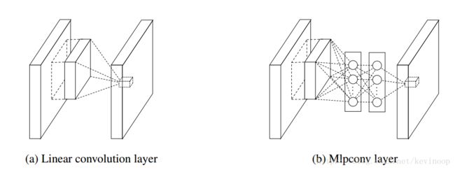
MLP Convolution Layers :
The resulting structure which we call an mlpconv layer is compared with CNN in picture below:
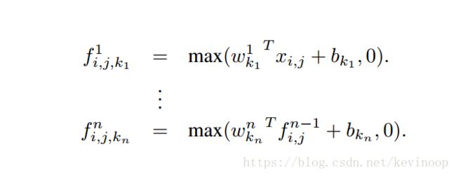
The feature maps are obtained by sliding the MLP over the input in a similar manner as CNN and fed into the next layer. Using the relu as an example represents the classic CNN, the feature map can be calculated as follows:
Maximization over linear functions makes a piecewise linear approximator which is capable of approximating any convex functions. Compared to conventional convolutional layers which perform linear separation, the maxout network is more potent as it can separate concepts that lie within convex sets.
The feature maps of maxout layers are calculated as follows:
We seek to achieve this by introducing the novel “Network In Network” structure, in which a micro network is introduced within each convolutional layer to compute more abstract features for local patches.
The calculation performed by mlpconv layer is shown as follows:
The following picture is prone to understanding:
(Statement: The picture is transfered form others)
Global Average Pooling :
Conventional convolutional neural networks perform convolution in the lower layers of the network. For classification, the feature maps of the last convolutional layer are vectorized and fed into fully connected layers followed by a softmax logistic regression layer. In this paper, we propose another strategy called global average pooling to replace the traditional fully connected layers in CNN.
The idea is to generate one feature map for each corresponding category of the classification tasks in the last mlpconv layer. Instead of adding fully connection layers , we take the average of each feature map, and the resulting vector fed directly into the softmax layer.
The disadvantage of fully connection layers:
too many parameters
be prone to over-fitting
The advantage of global average pooling:
- more native
- no parameters to optimize
- sums out the spatial information, thus it is more robust to spatial transformation of the input.
2.3.4 Inception V3
General Design Principles:
Avoid representational bottlenecks, especially early in the network. Theoretically, information content can not be assessed merely by the dimensionality of the representation as it discards important factors like correlation structure; the dimensionality merely provides a rough estimate of information content.
Higher dimensional representations are easier to process locally within a network.
Spatial aggregation can be done over lower dimensional embeddings without much or any loss in representational power.
Balance the width and depth of the network. The computational budget should therefore be distributed in a balanced way between the depth and width of the network.
Factorizing Convolutions with Large Filter Size:
Two ways to factorize convolution:
- Sliding this small network over the input activation grid boils down to replacing the 5 × 5 convolution with two layers of 3 × 3 convolution .
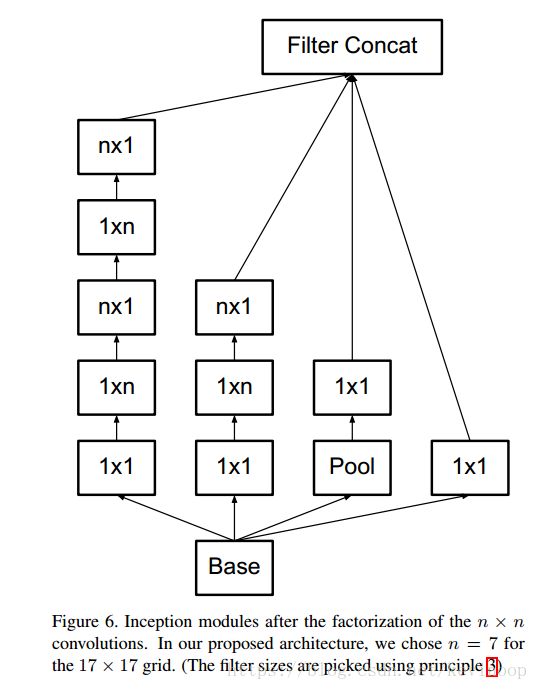
- using a 3 × 1 convolution followed by a 1 × 3 convolution is equivalent to sliding a two layer network with the same receptive field as in a 3 × 3 convolution .
We can get:
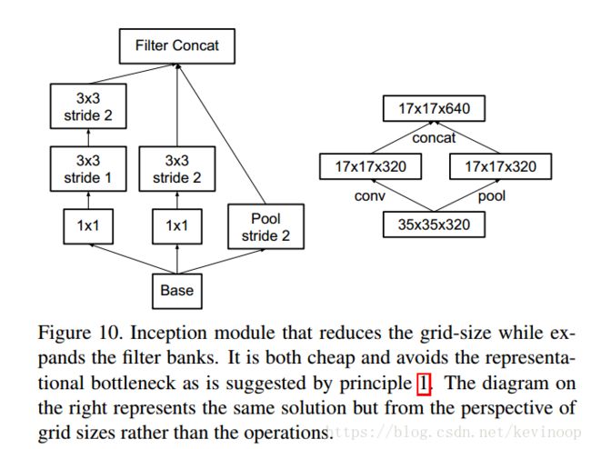
Efficient Grid Size Reduction :
We can use two parallel stride 2 blocks: P and C. P is a pooling layer (either average or maximum pooling) the activation, both of them are stride 2 the filter banks of which are concatenated as in figure [10].
Inception-v2 :
Model Regularization via Label Smoothing :
For each training example x, our model computes the probability of each label k , p(k|x)=ezk∑Ki=1ezi p ( k | x ) = e z k ∑ i = 1 K e z i . Consider the ground-truth distribution over labels q(k|x) q ( k | x ) for this training example, normalized so that ∑Ki=1q(k|x)=1 ∑ i = 1 K q ( k | x ) = 1 .
cross-entropy : l=−∑Kk=1log(p(k))q(k) l = − ∑ k = 1 K l o g ( p ( k ) ) q ( k ) .
Consider a distribution over labels u(k) u ( k ) , independent of the training example x, and a smoothing parameter ϵ ϵ . For a training example with ground-truth label y, we replace the label distribution q(k|x)=δk,y q ( k | x ) = δ k , y with
we used the uniform distribution u(k)=1/K u ( k ) = 1 / K , δk,y=q(x) δ k , y = q ( x ) (which equals 1 for k = y and 0 otherwise. )
Training Methodology :
batch_size=32, RMSProp decay=0.9, ϵ=1.0 ϵ = 1.0 . learning_rate-0.045, decayed every two epoch using an exponential rate of 0.94 ,gradient threshold 2.0.
2.3.5 ResNet- Deep Residual Learning for Image Recognition
There exists a solution by construction to the deeper model: the added layers are identity mapping , and the other layers are copied from the learned shallower model.
Formally, denoting the desired underlying mapping as H(x) H ( x ) ,we let the stacked nonlinear layers fit another mapping of F(x):=H(x)−x F ( x ) := H ( x ) − x . The original mapping is recast into F(x)+x F ( x ) + x .
We consider a building block defined as:
Here x and y are the input and output vectors of the layers considered. As shown above, there are two layers, F=w2σ(w1x) F = w 2 σ ( w 1 x ) in which σ σ denotes Relu and the biases are omitted for simplifying notations. The dimensions of x and F must be equal in Eqn.(3). If this is not the case (e.g., when changing the input/output channels), we can perform a linear projection Ws W s by the shortcut connections to match the dimensions:
Architectures for ResNet :
Deeper Bottleneck Architectures :
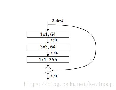
Next we describe our deeper nets for ImageNet. Because of concerns on the training time that we can afford, we modify the building block as a bottleneck design. For each residual function F, we use a stack of 3 layers instead of 2 . The three layers are 1×1, 3×3, and 1×1 convolutions, where the 1×1 layers are responsible for reducing and then increasing (restoring)
dimensions, leaving the 3×3 layer a bottleneck with smaller input/output dimensions. An example as shown below, where both designs have similar time complexity.
3 Neural Style Transfer
3.1 A Neural Algorithm of Artistic Style(L. A. Gatys)
a[l][C]ij a i j [ l ] [ C ] is the activation of the ith i t h filter at position j j in layer l l of content image.
Let C C and G G be the original image and the image that is generated .
- G[l][S]kk′ G k k ′ [ l ] [ S ] and G[l][G]kk′ G k k ′ [ l ] [ G ] give these feature correlations which is the inner product between the feature map k k and k′ k ′ in layer l l .
- ωl ω l are weighting factors of the contribution of each layer to the total loss .
- n[l]Hn[l]Wn[l]C n H [ l ] n W [ l ] n C [ l ] give the feature map the height, width and the number of channels.
α α and β β are the weighting factors for content and style reconstruction respectively.
4 Autoencoder
4.1 Stacked Denoising Autoencoders: Learning Useful Representations …
All appear build on the same principle that we may summarize as follows:
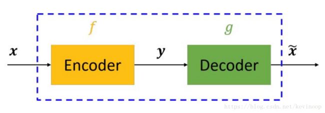
Traditional Autoencoders (AE) :
The Denoising Autoencoder Algorithm
The key difference is that z z is now a deterministic function of x^ x ^ rather than x x
We emphasize here that our goal is not the task of denoising per se. Rather denoising is advocated and investigated as a training criterion for learning to extract useful features that will constitute better higher level representation. The usefulness of a learnt representation can then be assessed objectively by measuring the accuracy of a classifier that uses it as input.
Geometric Interpretation
Stacking denoising autoencoders
Fine-tuning of a deep network for classification


