一、【python计算机视觉编程】基本的图像操作和处理

说明：本章介绍了python图像处理所需要的工具包，包括PIL，Matplotlib，Numpy，Scipy。本人比较喜欢用Matplotlib，因为它的语法与matlab比较相似。

（一）PIL：python图像处理类库

特别说明：PIL（图像处理类库）这个工具包只能用于python2.x的版本，目前该工具包也已经停止更新了。感兴趣的读者可以在下面的网站下载试试，在本篇博客中，用pillow工具包代替PIL工具，pillow不仅可以在python3.x的编辑器中使用，也兼容python2.x。读者可以在下载并安装anaconda后，使用Anaconda Prompt中进行下载安装：pip install pillow即可。

http://www.pythonware.com/products/pil/ PIL下载网站

虽然用pillow代替了PIL，但是所用的功能基本是不变的。

基本操作如下：

from PIL import Image    #每个代码的开头

• 打开一幅图像，这幅图需要和.py文件放在同目录下

from PIL import Image

#打开一幅图像，同时这幅图需要和.py文件放在同目录下
im=Image.open('apple.png')    
im.show()
#读取一幅图像，并将它转换为灰度图像
im_change=Image.open('apple.png').convert('L') 
im_change.show()

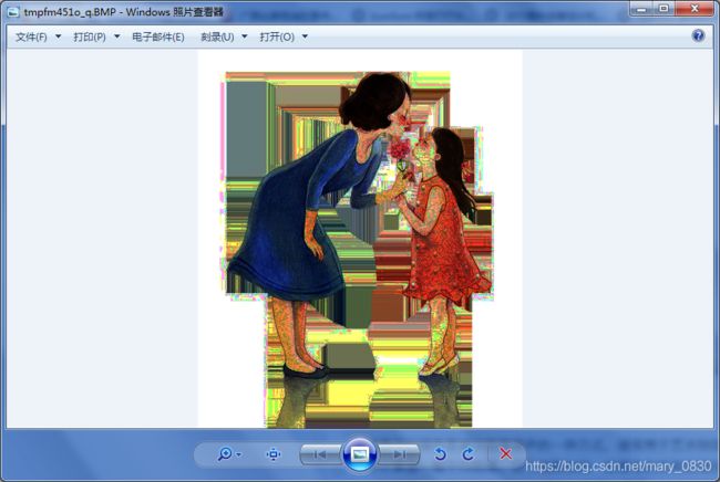
需要注意的是，如果没有安装xv，该函数甚至不能工作。由于实验是在安装win7系统的电脑上完成的，应该要设置windows 照片查看器为默认的程序，这样就可以运用show()查看所显示的图像。 如下图所示，是在windows照片查看器中显示的。

• 转换图像为jpg格式

from PIL import Image
import os

for infile in filelist:
    outfile=os.path.splitext(infile)[o]+".jpg"
    if infile !=outfile:
        try:
            Image.open(infile).save(outfile)
        except IOError:
            print "cannot convert",infile
            
def get_imlist(path):
    """返回目录中所有JPG图像的文件名列表"""
    return [os.path.join(path,f) for f in os.listdir(path) if f.endswith('.jpg')]

编写实验代码为：

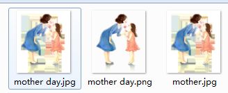
from PIL import Image
im = Image.open("mother day.png")
print(im)
im.save("mother day.jpg")     ## 将"mother day.png"保存为"mother day.jpg"
im = Image.open("mother day.jpg")  ##打开新的jpg图片
print(im.format, im.size, im.mode)

运行上面代码后，显示了一条错误：OSError: cannot write mode RGBA as JPEG。通过百度查询出错的原因，最后找到了。这是因为 ：RGBA意思是红色、绿色、蓝色、Alpha的色彩空间，而Alpha指透明度。而JPG不支持透明度，所以要么丢弃Alpha,要么保存为.png文件。 因此上面的代码可以用于将JPG图像转换成PNG图像，而不能倒过来转换。

通过修改实验代码，下面的代码可以完成图像PNG变成JPG图像之间转换：

im=im.convert('RGB')
im.save('mother day.jpg')

• 创建缩略图

im.thumbnail((128,128))  

这个操作比较简单，就把图像设置为想要的缩略图的尺寸即可。比如在上面代码中，把图像压缩成128*128像素。

• 复制和粘贴图像区域

crop() 的操作是从原始图像中返回一个矩形区域的拷贝，变量box是一个四元组，定义了左、上、右、下的像素坐标。为了获取一个分离的拷贝，可以调用load()操作对裁剪的图像进行拷贝。

编写裁剪的实验代码：

from PIL import Image

im = Image.open("mother day.jpg")
box = (100, 100, 300, 200)           #设定一块区域，分别是左上右下
region = im.crop(box)                #从一幅图中裁剪指定区域
region.show()     #显示被裁剪的区域

region=region.transpose(Image.ROTATE_180)   #旋转获取的区域
im.paste(region,box)   #用paste()将该区域粘贴回去

paste() 是将一张图粘贴到另一张图像上。变量box或者是一个给定左上角的二元组，也可以是定义了左、上、右、下像素坐标的四元组，或者为空（0,0）。如果给定四元组，被粘贴的图像的尺寸必须与区域尺寸一样。如果模式不匹配，被粘贴的图像将被转换为当前图像的模式。

编写裁剪复制后再粘贴回原图的代码：

from PIL import Image

im = Image.open("mother day.jpg")
box=(0,0,100,100)
im_crop = im.crop(box)
print(im_crop.size,im_crop.mode)
im.paste(im_crop, (100,100))          
im.paste(im_crop, (400,400,500,500))
im.show()

• 调整尺寸和旋转

out=im.resize((128,128))    #重设图像的大小，设为128*128像素
out1=im.rotate(45)   #将图像进行45°旋转

• 用透明图层复合在另一幅图上

from PIL import Image

im1 = Image.open('pineapple.png')
im2 = Image.open('watermelon.png')
im = Image.alpha_composite(im1,im2)
im.show()

• 复制图像

from PIL import Image
im = Image.open("mother day.jpg")
im_copy = im.copy()
im.save("mother.jpg")

（二）Matplotlib

说明：Matplotlib这个类库可以很好地处理数学运算、绘制图表、或者在图像上绘制点、直线和曲线等。Matplotlib是开源工具，可以从网站上免费下载。这个类库与matlab的有些语法很相似，适合刚刚学习过matlab的读者运用。

http://matplotlib.sourceforge.net/

（1）绘制图像、点和线

基本的代码如下所示，

from PIL import Image
from pylab import *

#读取图像到数组中
im=array(Image.open('apple.png'))

#绘制图像
imshow(im)

#设置点
x=[100,100,400,400]
y=[200,500,200,500]

#使用红色星状标记绘制点
plot(x,y,'r*')

#绘制连接前两个点的线
plot(x[:2],y[:2])

#添加标题，显示绘制的图像
title('plotting:"lemon.png"') 
show()

根据上面编写实验代码：

import matplotlib.pyplot as plt     # plt 用于显示图片
import matplotlib.image as mpimg     # mpimg 用于读取图片
import numpy as np  
 
lemon = mpimg.imread('lemon.png')     # 读取和代码处于同一目录下的图像
# 此时图像就已经是一个 np.array 了，可以对它进行任意处理
lemon.shape     #(512, 512, 3)
 
plt.imshow(lemon) # 显示图片
plt.axis('off') # 不显示坐标轴
plt.plot(100,50,'b*')     #使用蓝色星状标记绘制点
plt.plot(x[:2],y[:2])    #绘制连接前两个点的线
plt.title('plotting:"lemon.png"')    #添加标题，显示绘制的图像
plt.show()

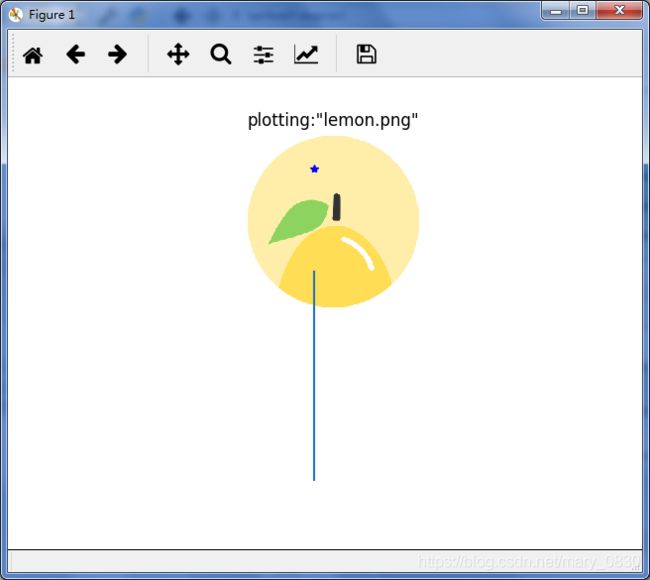
需要注意的是，当使用import matplotlib.pyplot as plt时，对图像plt进行操作，即每一步都需要plt.+操作的形式，如plt.imshow()，这样才能将某种操作作用于图像。

（2）图像轮廓和直方图

from PIL import Image
from pylab import *

#读取图像到数组中
im=array(Image.open('apple.png').convert('L'))

#新建一个图像
figure()

#变成灰度图像
gray()

#在原点的左上角显示轮廓图像
contour(im,origin='image')
axis('equal')
axis('off')

#绘制直方图
hist(im.flatten(),128)    #第二个参数指定小区间的数目
show()

在网上查询到了matplotlib.pyplot.hist的定义：

matplotlib.pyplot.hist(x, bins=None, range=None, normed=False, weights=None, cumulative=False, bottom=None, histtype='bar', align='mid', orientation='vertical', rwidth=None, log=False, color=None, label=None, stacked=False, hold=None, data=None, **kwargs)

根据上面编写实验代码，为了实现将图像的灰度化、绘制轮廓：

import matplotlib.pyplot as plt   # plt 用于显示图片
import matplotlib.image as mpimg # mpimg 用于读取图片
import numpy as np
 
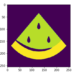
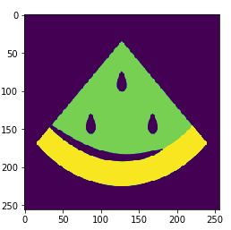
watermelon = mpimg.imread('watermelon.png')

def rgb2gray(rgb):     #定义RGB 图转换为灰度图的函数
    return np.dot(rgb[...,:3], [0.299, 0.587, 0.114])
 
gray = rgb2gray(watermelon)    
# 也可以用 plt.imshow(gray, cmap = plt.get_cmap('gray'))
plt.contour(gray,origin='image')
plt.axis('equal')
plt.imshow(gray, cmap='Greys_r')
plt.axis('off')
plt.show()

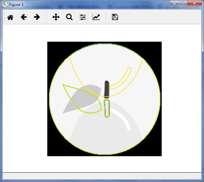
结果显示如上，发现轮廓与原始图像相反，但我没有得出其原因。

下面编写绘制图像直方图的代码：

import matplotlib.pyplot as plt   # plt 用于显示图片
import matplotlib.image as mpimg # mpimg 用于读取图片
import numpy as np
 
watermelon = mpimg.imread('watermelon.png')

#绘制直方图
#x =watermelon.shape
plt.hist(watermelon.flatten(),10,histtype='bar',facecolor='yellowgreen',alpha=0.8,rwidth=0.9)   
plt.xlabel("x")
plt.ylabel('y')
plt.title('hist')
plt.show()

（3）交互式标注

当用户需要和某些应用交互时，比如说在一幅图像中标记一些点，或者标注一些训练数据。可以用pylab库中的ginput()函数实现交互式标记。

from PIL import Image
from pylab import *

im=array(Image.open('watermelon.png'))
imshow(im)
print('Please click 3 points')
x=ginput(3)    #ginput()可以实现交互式标记
print ('you clicked:',x)
show()

（三）Numpy

说明：Numpy是python 科学计算工具包，包含数组对象（用来表示向量、矩阵、图像等）以及线性代数函数，可以对数组进行重要的操作，比如说矩阵乘积、转置、解方程系统、向量乘积和归一化等。

（1）图像数组表示

Numpy中的数组对象是多维的，可以用来表示向量、矩阵和图像。数组中所有的元素必须具有相同的数据类型，创建数组对象时需要指定数据类型，否则数据类型会自动确定。

编写实验代码：

from PIL import Image
from numpy import *
from pylab import *

im=array(Image.open('mother day.jpg'))
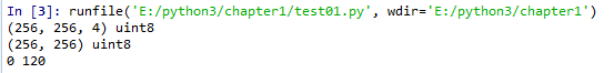
print (im.shape,im.dtype)

im=array(Image.open('mother day.jpg').convert('L'))
print (im.shape,im.dtype)

输出结果如下所示：


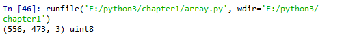
更换图像再进行一次运算得到的结果如下：

数组中的元素可以使用下标访问，位于坐标i,j,以及颜色通道k的像素值可以如下那样访问：value=im[i,j,k]
多个数组元素可以使用数组切片方式访问，切片方式返回的是以指定间隔下标访问该数组的元素值。需要注意的是，仅仅使用一个下标时，该下标是行下标。

下面是一些灰度图像的例子：

im[i,:]=im[j,:]   #将第k行的数值赋值给第i行
im[:,i]=100   #将第i列的所有数值设置为100
im[:100,:50].sum()   #计算前100行、前50列的所有数值的和
im[50:100,50:100]   #50~100行，50~100列所有数值的和
im[i].mean()   #第i行所有数值的平均值
im[:,-1]    #最后一列
im[-2,:](or im[-2])    #倒数第二行

（2）灰度变换

正如上面介绍的工具包，都会有把RGB图像变换成灰度图像，在这部分也介绍用Numpy把彩色图像变成灰度图像。

灰度变换的例子代码为：

from PIL import Image
from pylab import *
from numpy import *

im = array(Image.open("watermelon.png"))
print(im.shape,im.dtype)

im=array(Image.open("watermelon.png").convert('L'))
print(im.shape,im.dtype)

im2 = 255 - im       #对图像进行反相处理
figure()
imshow(im2)

im3 = (100.0/255)*im +100     #将图像像素值变换到100~200区间内
figure()
imshow(im3)

im4 = 255.0*(im/255.0)**2         #对图像的像素值求平方后得到的图像
figure()
imshow(im4)

print(int(im4.min()),int(im4.max()))    #输出像素的最大和最小值

show()

（反相处理图像）

（图像像素值变换到100~200区间）

（平方后得到的图像）

（3）图像缩放

想要对图像进行缩放处理并没有现成的方法，只能自定义函数imresize：

def imresize(im,sz):
    """使用PIL对象重新定义图像数组的大小"""
    pil_im = Image.fromarray(uint8(im))
    
    return array(pil_im.resize(sz))

（4）直方图均衡化

直方图均衡化是指将一幅图像的灰度直方图变平，使变换后的图像中每个灰度值的分布概率都相同，该方法可以增强图像的对比度。直方图均衡化的变换函数是图像中像素值的累计分布函数（cdf），将像素值的范围映射到目标范围的归一化操作。
首先介绍函数histeq用于处理直方图均衡化：

def histeq(im,nbr_bins=256):
    """对一幅灰度图像进行直方图均衡化"""
    
    #计算图像的直方图
    imhist,bins=histogram(im.flatten(),nbr_bins,normed=Ture)
    cdf=imhist.cumsum()   #cumulative distribution function
    cdf=255*cdf/cdf[-1]  #归一化
    
    #使用累计分布函数的线性插值，计算新的像素值
    im2=interp(im.flatten(),bins[:-1],cdf)
    
    return im2.reshape(im.shape),cdf

调用上面的函数所编写的实验代码：

from PIL import Image
from numpy import *
from pylab import *

im1 = Image.open("watermelon.png")   #打开原始图像
im_gray = im1.convert('L')     #变换为灰度图像
im_gray.show()         #显示灰度图像
im = array(Image.open('E:\Python\\fanwei.jpg').convert('L'))
# figure()
# hist(im.flatten(),256)
im2,cdf = histeq(im)
# figure()
# hist(im2.flatten(),256)
# show()
im2 = Image.fromarray(uint8(im2))
im2.show()
# print(cdf)
# plot(cdf)
im2.save("junheng.png")

实验过程中，出现了AttributeError: 'PngImageFile' object has no attribute 'flatten'的问题，上网查找问题的原因，说是png没有这个函数，那就将图像换成jpg类型的。但是还是出现了AttributeError: 'JpegImageFile' object has no attribute 'flatten'。最后在一位大神那找到了解决的方法：转换为数组array。

im1 = array（im,‘f’）# 由于可能对im1直接进行运算，对整型的像
                           #素数据的除运算，会导致小数丢失。故需要
                           #增加'f'option
arr = im1.flatten（） #将2D 数组变成一个一维数组 

重新编写代码为：

from PIL import Image
from numpy import *
from pylab import *

def histeq(im,nbr_bins=256):
    """对一幅灰度图像进行直方图均衡化"""
    
    #计算图像的直方图
    #在numpy中，也提供了一个计算直方图的函数histogram(),第一个返回的是直方图的统计量，第二个为每个bins的中间值
    imhist,bins=histogram(im.flatten(),nbr_bins,normed=1)
    cdf=imhist.cumsum()   #cumulative distribution function
    cdf=255*cdf / cdf[-1]  #归一化
    
    #使用累计分布函数的线性插值，计算新的像素值
    im2=interp(im.flatten(),bins[:-1],cdf)
    
    return im2.reshape(im.shape),cdf

im1 = Image.open("mother.jpg")   #打开原始图像
im_gray = im1.convert('L')     #变换为灰度图像
#im_gray.show()         #显示灰度图像

im = array(im1,'f')# 由于可能对im1直接进行运算，对整型的像
                           #素数据的除运算，会导致小数丢失。故需要
                           #增加'f'option
arr = im.flatten() #将2D 数组变成一个一维数组 
figure()
hist(arr,256)

im2,cdf = histeq(im)
figure()
hist(im2.flatten(),256)
show()

im2 = Image.fromarray(uint8(im2))
im2.show()
print(cdf)
plot(cdf)
im2.save("junheng.png")

（5）图像平均

图像平均操作是减少图像噪声的一种方式，通常用于艺术特效。可以简单地从图像列表中计算出一幅平均图像。这个函数包括一些基本的异常处理技巧，可以自动跳过不能打开的图像。也可以运用mean()函数计算平均图像，该函数需要将所有的图像堆积到一个数组中。

def compute_average(imlist):
""" 计算图像列表的平均图像"""
# 打开第一幅图像，将其存储在浮点型数组中
averageim = array(Image.open(imlist[0]), 'f')
for imname in imlist[1:]:
try:
averageim += array(Image.open(imname))
except:
print imname + '...skipped'
averageim /= len(imlist)
# 返回uint8 类型的平均图像
return array(averageim, 'uint8')

（6）图像的主成分分析（PCA）

图像的 主成分分析（PCA） 是一种降维的技巧，它可以在使用尽可能少维数的前提下，尽量多地保持训练数据的信息。可以把100*100像素的小灰度图像，看成10000维空间中的一个点。为了对图像数据进行PCA变换，图像需要转换成一维向量表示。

下面介绍PCA操作的代码，该函数通过减去每一维的均值将数据中心化，然后计算协方差矩阵对应最大特征值的特征向量，此时可以使用SVD分解。

from PIL import Image
from numpy import *

def pca(X):
    """主成分分析：
        输入：矩阵X，其中该矩阵中存储训练数据，每一行为一条训练数据
        返回：投影矩阵（按照维度的重要性排序）、方差和均值"""
        
        #获取维数
        num_data,dim=X.shape
        
        #数据中心化
        mean_X=X.mean(axis=0)
        X=X-mean_X
        
        if dim>num_data:
            #PCA-使用紧致技巧
            M=dot(X,X.T)  #协方差矩阵
            e,EV=linalg.eigh(M)   #特征值和特征向量
            tmp=dot(X.T,EV).T   #这就是紧致技巧
            V=tmp[::-1]   #由于最后的特征向量是我们所需要的，所以需要将其逆转
            S=squr(e)[::-1]  #由于特征值是按照递增顺序排列的，所以需要将其逆转
            for i in range(V.shape[1]):
                V[:,i]/=S
            else:
                #PCA-使用SVD方法
                U,S,V=linalg.svd(X)
                V=V[:num_data]  #仅仅返回前num_data维的数据才合理
                
                #返回投影矩阵、方差和均值
                return V,S,mean_X

对图像进行PCA变换，编写实验代码：

from PIL import Image
from numpy import *
from pylab import *
import pca

im=array(Image.open(imlist[o]))   #打开一幅图像，获取其大小
m,n=im.shape[0:2]  #获取图像的大小
imnbr=len(imlist)   #获取图像的数目

#创建矩阵，保存所有压平后的图像数据
immatrix=array([array(Image.open(im)).flatten() for im in imlist],'f')

#执行PCA操作
V,S,immean=pca.pca(immatrix)

#显示一些图像（均值图像和前7个模式）
figure()
gray()
subplot(2,4,1)
imshow(immean.reshape(m,n))
for i in range(7):
subplot(2,4,i+2)
imshow(V[i].reshape(m,n))

show()

当运行上面的代码时，出现了如下的报错：

 subplot(2,4,i+2)
          ^
IndentationError: expected an indented block

上面的意思是子位置（2,4，i+2）^缩进错误：需要缩进块。 需要注意的是，Python编辑器对文件格式是有严格的要求的，需要核对格式问题，如tab和空格没对齐，你需要检查下tab和空格了。但是经过检查tab和空格，以及代码的调整，依然还没有能够解决这个问题：

    return V,S,mean_X
                     ^
SyntaxError: 'return' outside function

求大佬帮我解决一下！！

（7）使用pickle模块

pickle模块可以接受几乎所有的python对象，并且将其转换成字符串表示，这个过程叫做封装。从字符串表示中重构该对象，叫做拆封。这些字符串表示可以方便地存储和传输。多个对象可以保存在同一个文件中，pickle模块中由很多不同的协议可以生成.pkl文件。在其他Python会话中载入数据，需要使用函数load()即可。

http://docs.python.org/library/pickle.html #pickle模块文档

编写实验代码：（保存上面图像的平均图像和主成分）

#保存均值和主成分数据
f=open('font_pca_modes.pkl','wb')
pickle.dump(immean,f)
pickle.dump(V,f)
f.close()

#载入均值和主成分数据
f=open('font_pca_modes.pkl','rb')
immean=pickle.load(f)
V=pickle.load(f)
f.close()

savetxt('test.txt',x,'%i')    #保存一个数组x到文件里

x=loadtxt('test.txt')   #读取数组x

# 打开文件并保存
with open('font_pca_modes.pkl', 'wb') as f:
pickle.dump(immean,f)
pickle.dump(V,f)

# 打开文件并载入
with open('font_pca_modes.pkl', 'rb') as f:
immean = pickle.load(f)
V = pickle.load(f)

（四）Scipy

Scipy工具包是建立载Numpy基础之上的，用于数值运算的开源工具包，可以实现数值积分、优化、统计、信号处理，以及图像处理。可以用如下的网址进行下载。

http://scipy.org/Download

（1）图像模糊

图像模糊就是将灰度图像I和一个高斯核进行卷积的操作：

其中，*表示卷积操作。

这是二维高斯核的定义。高斯模糊通常是其他图像处理操作的一部分，就是之前学习冈萨雷斯那本书的高斯滤波类似，把尖锐的部分或者断裂的部分，可以通过滤波去平滑图像的操作。

from PIL import Image
from numpy import *
from scipy.ndimage import filters

im = array(Image.open('empire.jpg').convert('L'))
im2 = filters.gaussian_filter(im,5)

im = array(Image.open('empire.jpg'))
im2 = zeros(im.shape)
for i in range(3):
im2[:,:,i] = filters.gaussian_filter(im[:,:,i],5)
im2 = uint8(im2)

（2）图像导数

图像的强度变换是图像处理中的重要一步，强度的变换可以用灰度图像I（对于彩色图像来说，对每个颜色通道分别计算导数）的x和y方向导数Ix和Iy进行描述。图像的梯度向量为

梯度由两个属性组成：一是梯度的大小，描述图像强度变换的强弱；二是梯度的角度，描述了图像中在每个点上强度变换最大的方向。数学表达式如下所示：

from PIL import Image
from numpy import *
from scipy.ndimage import filters

im = array(Image.open('empire.jpg').convert('L'))

# Sobel 导数滤波器
imx = zeros(im.shape)
filters.sobel(im,1,imx)

imy = zeros(im.shape)
filters.sobel(im,0,imy)

magnitude = sqrt(imx**2+imy**2)

filters.gaussian_filter() 函数可以接受额外的参数，用来计算高斯导数。

sigma = 5 # 标准差

imx = zeros(im.shape)
filters.gaussian_filter(im, (sigma,sigma), (0,1), imx)

imy = zeros(im.shape)
filters.gaussian_filter(im, (sigma,sigma), (1,0), imy)

（3）形态学：对象计数

形态学是度量和分析基本形状的图像处理方法的基本框架与集合。通常用于处理二值图像，也可以用于处理灰度图像。二值图像通常是在计算物体的数目或者度量其大小时，对一幅图像进行阈值化后的结果。scipy.ndimage中的morphology模块可以实现形态学的操作。还提供measurements模块来实现二值图像的计数和度量功能。

from scipy.ndimage import measurements,morphology

# 载入图像，然后使用阈值化操作，以保证处理的图像为二值图像
im = array(Image.open('houses.png').convert('L'))
im = 1*(im<128)

labels, nbr_objects = measurements.label(im)
print "Number of objects:", nbr_objects

# 形态学开操作更好地分离各个对象
im_open = morphology.binary_opening(im,ones((9,5)),iterations=2)

labels_open, nbr_objects_open = measurements.label(im_open)
print "Number of objects:", nbr_objects_open

（4）一些有用的Scipy模块：io和misc

• 读写.mat文件
  当有数据是以matlab的.mat文件格式存储，可以使用scipy.io模块进行读取。
  data=scipy.io.loadmat('test.mat')

当需要保存所需要的变量时，即创建一个字典，可以使用savemat()函数：

data={}
data['x']=x
scipy.io.savemat('test.mat',data)

• 以图像形式保存数组
  当需要对图像进行操作时，需要使用数组对象来做运算，所以将数组直接保存为图像文件是非常有用的。imsave()函数可以从scipy.misc模块中载入，要将数组im保存到文件中，可以进行如下操作：

from scipy.misc import imsave
imsave('test.jpg',im)
lena=scipy.misc.lena()

（五）高级示例：图像去噪

ROF去噪模型，使处理后的图像更加平滑，同时保持图像边缘和结构信息。简要介绍ROF模型：
一幅灰度图像I的全变差（TV）定义为梯度范数之和。在连续表示的情况下，全变差表示为：

在离散表示的情况下，全变差表示为：

其中，上面的式子是在所有图像坐标x=[x,y]上取和。在Chambolle提出的ROF模型里，目标函数为寻找降噪后的图像U，使下式最小：

其中范数|| I-U ||是去噪后图像U和原始图像I差异的度量。本质上该模型使去噪后的图像像素值“平坦”变化，但在图像区域的边缘上，允许去噪后的图像像素值“跳跃”变化。

from numpy import *

def denoise(im,U_init,tolerance=0.1,tau=0.125,tv_weight=100):
  """ 使用A. Chambolle（2005）在公式（11）中的计算步骤实现Rudin-Osher-Fatemi（ROF）去噪模型

    输入：含有噪声的输入图像（灰度图像）、U 的初始值、TV 正则项权值、步长、停业条件

    输出：去噪和去除纹理后的图像、纹理残留"""

m,n = im.shape # 噪声图像的大小

# 初始化
U = U_init
Px = im # 对偶域的x 分量
Py = im # 对偶域的y 分量
error = 1

while (error > tolerance):
  Uold = U

  # 原始变量的梯度
  GradUx = roll(U,-1,axis=1)-U # 变量U 梯度的x 分量
  GradUy = roll(U,-1,axis=0)-U # 变量U 梯度的y 分量

  # 更新对偶变量
  PxNew = Px + (tau/tv_weight)*GradUx
  PyNew = Py + (tau/tv_weight)*GradUy
  NormNew = maximum(1,sqrt(PxNew**2+PyNew**2))

  Px = PxNew/NormNew # 更新x 分量（对偶）
  Py = PyNew/NormNew # 更新y 分量（对偶）

  # 更新原始变量
  RxPx = roll(Px,1,axis=1) # 对x 分量进行向右x 轴平移
  RyPy = roll(Py,1,axis=0) # 对y 分量进行向右y 轴平移

  DivP = (Px-RxPx)+(Py-RyPy) # 对偶域的散度
  U = im + tv_weight*DivP # 更新原始变量

  # 更新误差
  error = linalg.norm(U-Uold)/sqrt(n*m);

return U,im-U # 去噪后的图像和纹理残余

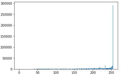
编写合成噪声图像的代码：

from numpy import *
from numpy import random
from scipy.ndimage import filters
import rof

# 使用噪声创建合成图像
im = zeros((500,500))
im[100:400,100:400] = 128
im[200:300,200:300] = 255
im = im + 30*random.standard_normal((500,500))

U,T = rof.denoise(im,im)
G = filters.gaussian_filter(im,10)

# 保存生成结果
from scipy.misc import imsave
imsave('synth_rof.pdf',U)
imsave('synth_gaussian.pdf',G)

保存好的结果：
在实际图像中使用ROF模型去噪声的实验代码如下：

from PIL import Image
from pylab import *
import rof

im = array(Image.open('watermelon.png').convert('L'))
U,T = rof.denoise(im,im)

figure()
gray()
imshow(U)
axis('equal')
axis('off')
show()

第一次运行程序时，就出现了如下的错误：
通过上网找资料，找到了原因，那就是：书上的代码是错误的。

需要的是，把def denoise定义成如下：

def denoise(im, U_init, tolerance=0.1, tau=0.125, tv_weight=100):
    """ An implementation of the Rudin-Osher-Fatemi (ROF) denoising model
        using the numerical procedure presented in Eq. (11) of A. Chambolle
        (2005). Implemented using periodic boundary conditions 
        (essentially turning the rectangular image domain into a torus!).
    
        Input:
        im - noisy input image (grayscale)
        U_init - initial guess for U
        tv_weight - weight of the TV-regularizing term
        tau - steplength in the Chambolle algorithm
        tolerance - tolerance for determining the stop criterion
    
        Output:
        U - denoised and detextured image (also the primal variable)
        T - texture residual"""
    
    #---Initialization
    m,n = im.shape #size of noisy image

    U = U_init
    Px = im #x-component to the dual field
    Py = im #y-component of the dual field
    error = 1 
    iteration = 0

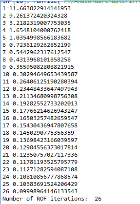
    #---Main iteration
    while (error > tolerance):
        Uold = U

        #Gradient of primal variable
        LyU = vstack((U[1:,:],U[0,:])) #Left translation w.r.t. the y-direction
        LxU = hstack((U[:,1:],U.take([0],axis=1))) #Left translation w.r.t. the x-direction

        GradUx = LxU-U #x-component of U's gradient
        GradUy = LyU-U #y-component of U's gradient

        #First we update the dual varible
        PxNew = Px + (tau/tv_weight)*GradUx #Non-normalized update of x-component (dual)
        PyNew = Py + (tau/tv_weight)*GradUy #Non-normalized update of y-component (dual)
        NormNew = maximum(1,sqrt(PxNew**2+PyNew**2))

        Px = PxNew/NormNew #Update of x-component (dual)
        Py = PyNew/NormNew #Update of y-component (dual)

        #Then we update the primal variable
        RxPx =hstack((Px.take([-1],axis=1),Px[:,0:-1])) #Right x-translation of x-component
        RyPy = vstack((Py[-1,:],Py[0:-1,:])) #Right y-translation of y-component
        DivP = (Px-RxPx)+(Py-RyPy) #Divergence of the dual field.
        U = im + tv_weight*DivP #Update of the primal variable

        #Update of error-measure
        error = linalg.norm(U-Uold)/sqrt(n*m);
        iteration += 1;

        print (interation, error)

    #The texture residual
    T = im - U
    print( 'Number of ROF iterations: ', iteration)
    
    return U,T