[通过scikit-learn掌握机器学习] 02 线性回归

【 http://blog.csdn.net/u013719780/article/details/51742982】  

   本章介绍用线性模型处理回归问题。回归问题的目标是预测出响应变量的连续值。

    

     从简单问题开始，先处理一个响应变量和一个解释变量的一元问题。同时讲一下如何做模型评估。

     然后，我们介绍多元线性回归问题（multiple linear regression），线性约束由多个解释变量构成。

     再之后，我们介绍多项式回归分析（polynomial regression问题），一种具有非线性关系的多元线性回归问题。

     最后，我们介绍如果训练模型获取目标函数最小化的参数值。

     在研究一个大数据集问题之前，我们先从一个小问题开始学习建立模型和学习算法。

---

一元线性回归

     假设你想计算匹萨的价格。

     虽然看看菜单就知道了，不过也可以用机器学习方法建一个线性回归模型， 通过分析匹萨的直径与价格的数据的线性关系，来预测任意直径匹萨的价格。

     我们先用scikit-learn写出回归模型，然后我们介绍模型的用法，以及将模型应用到具体问题中。假设我们查到了部分匹萨的直径与价格的数据，这就构成了训练数据，如下表所示：

训练样本	直径（英寸）	价格（美元）
1	6	7
2	8	9
3	10	13
4	14	17.5
5	18	18

     我们可以用matplotlib画出图形：

import matplotlib.pyplot as plt def run_plt():     plt.figure()     plt.title('Price-Size')     plt.xlabel('Size')     plt.ylabel('Price')     plt.axis([0, 25, 0, 25])     plt.grid(True)     return plt plt = run_plt() X = [[6], [8], [10], [14], [18]] y = [[7], [9], [13], [17.5], [18]] plt.plot(X, y, 'k.') plt.show()

     能够看出，匹萨价格与其直径正相关，这与我们的日常经验也比较吻合，自然是越大越贵。下面我们就用scikit-learn来构建模型。

from sklearn.linear_model import LinearRegression X = [[6], [8], [10], [14], [18]] y = [[7], [9], [13], [17.5], [18]] model = LinearRegression() model.fit(X, y) print('Predict the price by linear regression: $%.2f' % model.predict([12])[0])

     一元线性回归假设解释变量和响应变量之间存在线性关系；

      这个线性模型所构成的空间是一个超平面（hyperplane）。超平面是n维欧氏空间中余维度等于一的子空间，总比包含它的空间少一维。

     在一元线性回归中，一个维度是响应变量，另一个维度是解释变量，总共两维。因此，其超平面只有一维，就是一条线(直线或者曲线，具体要看选取的回归函数)。

     上述代码中sklearn.linear_model.LinearRegression是一个 估计器（estimator）。估计器依据观测值来预测结果。在scikit-learn里面，所有的估计器都带有fit()和predict()方法。fit()用来通过训练数据来确认模型需要的参数，predict()是通过模型对解释变量进行预测。

     因为所有的估计器都有这两种方法，所有scikit-learn很容易实验不同的模型。

     LinearRegression类的fit()方法学习下面的一元线性回归模型： y = α + βx。截距 α 和相关系数 β 是线性回归模型最关心的事情。

     y 表示响应变量的预测值，本例指匹萨价格预测值， x 是解释变量，本例指匹萨直径。下图中的直线就是匹萨直径与价格的线性关系。用这个模型，你可以计算不同直径的价格。

      实际上由于  y = α + βx 只需要两组输入[x,y]就能够之际计算一条之间，但是我们给定的数据要大于两组，因此每两两组合可以算出很多条直线。那么就涉及到在这么多直线中选哪一条的问题。也就是，这个方程是模型，而训练数据让我们可以选择合理的模型参数。

# coding=utf-8 import matplotlib.pyplot as plt from sklearn.linear_model import LinearRegression def run_plt():     plt.figure()     plt.title('Price-Size')     plt.xlabel('Size')     plt.ylabel('Price')     plt.axis([0, 25, 0, 25])     plt.grid(True)     return plt x = [[6], [8], [10], [14], [18]] y = [[7], [9], [13], [17.5], [18]] model = LinearRegression() model.fit(x, y) plt = run_plt() x2 = [[0], [10], [14], [25]] y2 = model.predict(x2) plt.plot(x, y, '.')  # 最后一个参数指定绘图类型，'.' 为点 plt.plot(x2, y2, '-')  # 最后一个参数指定绘图类型，'.' 为点 plt.show()

     一元线性回归拟合模型的参数估计常用方法是普通最小二乘法（ordinary least squares ）或线性最小二乘法（linear least squares）。

      首先，我们定义出拟合成本函数，然后对参数进行数理统计。成本函数（cost function）也叫损失函数（loss function），用来定义模型与观测值的误差。模型预测的价格与 训练集 数据的差异称为残差（residuals）或训练误差（training errors）。

      后面我们会用模型计算 测试集 ，那时模型预测的价格与测试集数据的差异称为预测误差（prediction errors）或训练误差（test errors）。

     模型的残差是训练样本点与线性回归模型的纵向距离，如下图所示：

……. plt = run_plt() x2 = [[0], [10], [14], [25]] model = LinearRegression() model.fit(x, y) y2 = model.predict(x2) plt.plot(x, y, '.') plt.plot(x2, y2, '-') # 用模型来预测训练输入，为了得到残差 yr = model.predict(x)   # 将原始值与模型算出来的值之间连线， 每个输入都对应一条短线 for idx, i in enumerate(x):       plt.plot([i, i], [y[idx], yr[idx]], 'r-')  # r 指的是 red, 表明这些线是红色的 plt.show()

     我们可以通过残差之和最小化实现最佳拟合，也就是说模型预测的值与训练集的数据最接近就是最佳拟合。 对模型的拟合度进行评估的函数称为残差平方和（residual sum of squares）成本函数。就是让所有训练数据与模型的残差的平方之和最小化，如下所示：

                           

其中， y i 是观测值， f ( x i )   是预测值。

     有了成本函数，就要使其最小化从而确定模型中的参数。 解一元线性回归的最小二乘法。 

     通过成本函数最小化获得参数，我们先求相关系数 β 。按照频率论的观点，我们首先需要计算 x 的方差和 x 与 y 的协方差。

方差是用来衡量样本分散程度的。如果样本全部相等，那么方差为0。方差越小，表示样本越集中，反正则样本越分散。 其中， x ¯ 是直径 x 的均值， x i 的训练集的第 i 个直径样本， n 是样本数量。	Numpy里面有 var 方法可以直接计算方差， ddof 参数是贝塞尔(无偏估计)校正系数（Bessel's correction），设置为1，可得样本方差无偏估计量。 import numpy as np (np . var([ 6 ,  8 ,  10 ,  14 ,  18 ],ddof = 1 ))
协方差表示两个变量的总体的变化趋势。 如果两个变量的变化趋势一致，那么两个变量之间的协方差就是正值。 如果两个变量的变化趋势相反，那么两个变量之间的协方差就是负值。如果两个变量不相关，则协方差为0。 变量线性无关不表示一定没有其他相关性。 其中， x ¯ 是直径 x 的均值， x i 的训练集的第 i 个直径样本， y ¯ 是价格 y 的均值， y i 的训练集的第 i 个价格样本， n 是样本数量。	Numpy里面有cov方法可以直接计算方差。 import numpy as np print(np.cov([6, 8, 10, 14, 18], [7, 9, 13, 17.5, 18])[0][1])
在一元线性回归中，有了方差和协方差，就可以计算相关系统 β 了。
算出 β 后，我们就可以计算 α 了

      这样就通过最小化成本函数求出模型参数了。把匹萨直径带入方程就可以求出对应的价格了。

---

模型评估

     如何评价模型在现实中的表现呢？现在让我们假设有另一组数据，作为测试集进行评估。

训练样本	直径（英寸）	价格（美元）	预测值（美元）
1	8	11	9.7759
2	9	8.5	10.7522
3	11	15	12.7048
4	16	18	17.5863
5	12	11	13.6811

     这里我们用R方（r-squared）评估匹萨价格预测的效果。 R方也叫确定系数（coefficient of determination），表示模型对现实数据拟合的程度。计算R方的方法有几种。一元线性回归中R方等于皮尔逊积矩相关系数（Pearson product moment correlation coefficient或Pearson's r）的平方。

     这种方法计算的R方一定介于0～1之间的正数。其他计算方法，包括scikit-learn中的方法，不是用皮尔逊积矩相关系数的平方计算的，因此当模型拟合效果很差的时候R方会是负值。

首先，我们需要计算样本总体平方和，y¯是价格y的均值，yi的训练集的第i个价格样本，n是样本数量。
我们计算残差平方和
最后计算R方：

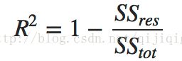
     R方是0.6620说明测试集里面过半数的价格都可以通过模型解释。现在，让我们用scikit-learn来验证一下。 LinearRegression的score方法可以计算R方：

from sklearn.linear_model import LinearRegression x = [[6], [8], [10], [14], [18]] y = [[7], [9], [13], [17.5], [18]] model = LinearRegression() model.fit(x, y) x_test = [[8], [9], [11], [16], [12]] y_test = [[11], [8.5], [15], [18], [11]] model = LinearRegression() model.fit(x, y) print model.score(x_test, y_test)

---

多元线性回归

     可以看出匹萨价格预测的模型R方值并不显著。如何改进呢？用一元线性回归已经无法解决了，我们可以用更具一般性的模型来表示，即多元线性回归。

     回顾一下自己的生活经验，匹萨的价格其实还会受到其他因素的影响。比如，匹萨的价格还与上面的辅料有关，所以让我们再为模型增加一个解释变量。

     增加辅料的匹萨价格预测模型训练集和测试集如下表所示： 

训练样本	直径（英寸）	辅料种类	价格（美元）
1	6	2	7
2	8	1	9
3	10	0	13
4	14	2	17.5
5	18	0	18
测试样本	直径（英寸）	辅料种类	价格（美元）
1	8	2	11
2	9	0	8.5
3	11	2	15
4	16	2	18
5	12	0	11

     同样通过最小二乘法，可以计算出参数，然后再看看 R 值。这里直接使用 LinearRegression 来进行计算了：

from sklearn.linear_model import LinearRegression X = [[6, 2], [8, 1], [10, 0], [14, 2], [18, 0]] y = [[7], [9], [13], [17.5], [18]] model = LinearRegression() model.fit(X, y) X_test = [[8, 2], [9, 0], [11, 2], [16, 2], [12, 0]] y_test = [[11], [8.5], [15], [18], [11]] predictions = model.predict(X_test) for i, prediction in enumerate(predictions):     print('Predicted: %s, Target: %s' % (prediction, y_test[i])) print('R-squared: %.2f' % model.score(X_test, y_test))

输出结果是： Predicted: [ 10.0625], Target: [11] Predicted: [ 10.28125], Target: [8.5] Predicted: [ 13.09375], Target: [15] Predicted: [ 18.14583333], Target: [18] Predicted: [ 13.3125], Target: [11] R-squared: 0.77

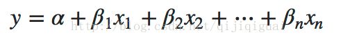
     现在我们可以认为，匹萨价格预测问题，多元回归确实比一元回归效果更好。假如解释变量和响应变量的关系不是线性的呢？下面我们来研究一个特别的多元线性回归的情况，可以用来构建非线性关系模型。

---

多项式回归

     上例中，我们假设解释变量和响应变量的关系是线性的。

     真实情况未必如此。下面我们用多项式回归，一种特殊的多元线性回归方法，增加了指数项。现实世界中的曲线关系都是通过增加多项式实现的，其实现方式和多元线性回归类似。本例还用一个解释变量，匹萨直径。让我们用下面的数据对两种模型做个比较：

训练样本	直径（英寸）	价格（美元）
1	6	7
2	8	9
3	10	13
4	14	17.5
5	18	18
测试样本	直径（英寸）	价格（美元）
1	6	8
2	8	12
3	11	15
4	16	18

     二次回归（Quadratic Regression），即回归方程有个二次项，公式：

     我们只用 一个解释变量，但是模型有三项，通过第三项（二次项）来实现曲线关系。实际上，我们可以换一个角度看这个问题， x^2 可以看做一个独立的变量，那么这就转变成了一个二元一次的问题。为了做掉这一点，需要将输入 x 转换一下, 一个输入变成两个，比如上例中输入为 [6,8,10,14,18] -->  [ [6, 36], [8, 64], [10, 100], [14, 196], [18, 324]]

                 

     上面的  就变成了二元一次线性拟合问题，之前讲过的 LinearRegression 就可以做了。

     而在PolynomialFeatures就可可以用来完成做输入扩展。

         

     代码如下：

from sklearn.preprocessing import PolynomialFeatures X_train = [[6], [8], [10], [14], [18]] quadratic_featurizer = PolynomialFeatures(2)  # 最多到二次方 X_train_quadratic = quadratic_featurizer.fit_transform(X_train) print (X_train_quadratic)

输出为： [[   1.    6.   36.]  [   1.    8.   64.]  [   1.   10.  100.]  [   1.   14.  196.]  [   1.   18.  324.]] 可以看到，就是对输入做了扩展， 从0次方最多到二次方

# coding=utf-8 import numpy as np from sklearn.linear_model import LinearRegression from sklearn.preprocessing import PolynomialFeatures import matplotlib.pyplot as plt def run_plt():     plt.figure()     plt.title('Price-Size')     plt.xlabel('Size')     plt.ylabel('Price')     plt.axis([0, 25, 0, 25])     plt.grid(True)     return plt plt = run_plt() X_train = [[6], [8], [10], [14], [18]] y_train = [[7], [9], [13], [17.5], [18]] X_test = [[6], [8], [11], [16]] y_test = [[8], [12], [15], [18]] # 返回一个数组，范围是 0 ~ 25, 共100个点, 这样可以画出预测出来的函数对应的线 xx = np.linspace(0, 25, 100)   xx_input = xx.reshape(xx.shape[0], 1)  # 转化成一个跟 X_train 内容一致的1*100的矩阵 print (xx_input) plt.plot(X_train, y_train, 'b.')  # 画原始的训练集的点 plt.plot(X_test, X_test, 'r.')  # 画原始的测试集的点 # 计算用一元一次线性回归出来的结果，然后画一条直线 regressor = LinearRegression() regressor.fit(X_train, y_train) yy = regressor.predict(xx_input) plt.plot(xx, yy, 'c-')  # 画一元一次回归对应的结果 print('Linear Regression r-squared', regressor.score(X_test, y_test)) # # quadratic 二次的 quadratic_featurizer = PolynomialFeatures(2) X_train_quadratic = quadratic_featurizer.fit_transform(X_train) X_test_quadratic = quadratic_featurizer.transform(X_test) print(X_train_quadratic)  # 转换过的输入 regressor_quadratic = LinearRegression() regressor_quadratic.fit(X_train_quadratic, y_train) xx_quadratic = quadratic_featurizer.transform(xx.reshape(xx.shape[0], 1)) # 画二元一次回归对应的结果，而这个二元实际上通过一元输入转换过来的 plt.plot(xx, regressor_quadratic.predict(xx_quadratic), 'm-')   print('Polynomial Regression r-squared', regressor_quadratic.score(X_test_quadratic, y_test)) plt.show()

从图形上看，一元二次由于是曲线，对训练集的拟合效果更好。 [[  0.        ]  [  0.25252525]  ……………….  [ 24.74747475]  [ 25.        ]] ('Linear Regression r-squared', 0.80972679770766498) [[   1.    6.   36.]  [   1.    8.   64.]  [   1.   10.  100.]  [   1.   14.  196.]  [   1.   18.  324.]] ('Polynomial Regression r-squared', 0.86754436563451076) 注：  二次拟合的 R 值要高于 一次拟合。 但是，用上一个例子给出的测试集，也就是 X=[8,9,11,16,12] Y=[11,8.5,15.18.11] 来计算 R 值，可以得到，其实一次拟合的 R 值要高于二次拟合。 也就是说，R 值跟训练集和测试集同时相关，而且不能简单的说高次拟合就一定比低次拟合效果好。 后面我们会论述一个问题：为什么只用一个测试集评估一个模型的效果是不准确的，如何通过将测试集数据分块的方法来测试，让模型的测试效果更可靠。

     针对这个例子中的训练集和测试集，一次回归的 R 值而0.81，而二次回归的 R 值为0.86。所以我们可以考虑一下更高次的回归是不是效果更好。同样的，也是将一维的输入，扩展到多维，然后在用多元一次方程来线性拟合。

quadratic_featurizer = PolynomialFeatures(2) X_train_quadratic = quadratic_featurizer.fit_transform(X_train) X_test_quadratic = quadratic_featurizer.transform(X_test) regressor_quadratic = LinearRegression() regressor_quadratic.fit(X_train_quadratic, y_train) xx_quadratic = quadratic_featurizer.transform(xx.reshape(xx.shape[0], 1)) plt.plot(xx, regressor_quadratic.predict(xx_quadratic), 'm-') cubic_featurizer = PolynomialFeatures(3) X_train_cubic = cubic_featurizer.fit_transform(X_train) X_test_cubic = cubic_featurizer.transform(X_test) regressor_cubic = LinearRegression() regressor_cubic.fit(X_train_cubic, y_train) xx_cubic = cubic_featurizer.transform(xx.reshape(xx.shape[0], 1)) plt.plot(xx, regressor_cubic.predict(xx_cubic)) print(X_train_cubic) print('2 Polynomial r-squared', regressor_quadratic.score(X_test_quadratic, y_test)) print('3 Polynomial r-squared', regressor_cubic.score(X_test_cubic, y_test)) plt.show()

其中蓝色的是三次拟合的曲线，蓝色为二次拟合的曲线。可以看到对训练数据的拟合程度上，三次要好的多。 二次回归 r-squared 0.867544458591 三次回归 r-squared 0.835692454062

quadratic_featurizer = PolynomialFeatures(2) X_train_quadratic = quadratic_featurizer.fit_transform(X_train) X_test_quadratic = quadratic_featurizer.transform(X_test) regressor_quadratic = LinearRegression() regressor_quadratic.fit(X_train_quadratic, y_train) xx_quadratic = quadratic_featurizer.transform(xx.reshape(xx.shape[0], 1)) plt.plot(xx, regressor_quadratic.predict(xx_quadratic), 'm-') seventh_featurizer = PolynomialFeatures(7) X_train_seventh = seventh_featurizer.fit_transform(X_train) X_test_seventh = seventh_featurizer.transform(X_test) regressor_seventh = LinearRegression() regressor_seventh.fit(X_train_seventh, y_train) xx_seventh = seventh_featurizer.transform(xx.reshape(xx.shape[0], 1)) plt.plot(xx, regressor_seventh.predict(xx_seventh)) print('2 Polynomial r-squared', regressor_quadratic.score(X_test_quadratic, y_test)) print('7 Polynomial r-squared', regressor_seventh.score(X_test_seventh, y_test)) plt.show()

二次回归 r-squared 0.867544458591 七次回归 r-squared 0.487942421984

     可以看出，七次拟合的R方值更低，虽然其图形基本经过了所有的点。 可以认为这是拟合过度（over-fitting）的情况。这种模型并没有从输入和输出中推导出一般的规律，而是记忆训练集的结果，这样在测试集的测试效果就不好了。

---

正则化

      正则化（Regularization）是用来防止拟合过度的一堆方法。正则化向模型中增加信息，经常是一种对抗复杂性的手段。

     scikit-learn提供了一些方法来使线性回归模型正则化。其中之一是岭回归(Ridge Regression，RR，也叫Tikhonov regularization)，通过放弃最小二乘法的无偏性，以损失部分信息、降低精度为代价获得回归系数更为符合实际、更可靠的回归方法。岭回归增加L2范数项（相关系数向量平方和的平方根）来调整成本函数（残差平方和）：

λ 是调整成本函数的超参数（hyperparameter），不能自动处理，需要手动调整一种参数。 λ 增大，成本函数就变大。

scikit-learn也提供了最小收缩和选择算子(Least absolute shrinkage and selection operator, LASSO)，增加L1范数项（相关系数向量平方和的平方根）来调整成本函数（残差平方和）：

LASSO方法会产生稀疏参数，大多数相关系数会变成0，模型只会保留一小部分特征。而岭回归还是会保留大多数尽可能小的相关系数。当两个变量相关时，LASSO方法会让其中一个变量的相关系数会变成0，而岭回归是将两个系数同时缩小。

scikit-learn还提供了弹性网（elastic net）正则化方法，通过线性组合L1和L2兼具LASSO和岭回归的内容。可以认为这两种方法是弹性网正则化的特例。

---

梯度下降法拟合模型

    前面的内容都是通过最小化成本函数来计算参数的：

    这里X是解释变量矩阵，当变量很多（上万个）的时候，XTX计算量会非常大。另外，如果XTX的行列式为0，即奇异矩阵，那么就无法求逆矩阵了。

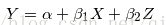
对于                        写成矩阵形式： Y  =  X β                    其中， Y 是训练集的响应变量列向量， β 是模型参数列向量。 X 称为设计矩阵，是 m×n 维训练集的解释变量矩阵。 m 是训练集样本数量， n 是解释变量个数。     在这里，我们的n为2， 即 我们的学习算法评估三个参数的值：两个相关因子和一个截距。     对于 Y = X β，矩阵没有除法运算（详见线性代数相关内容），所以用矩阵的转置运算和逆运算来实现：

     这里我们介绍另一种参数估计的方法，梯度下降法（gradient descent）。拟合的目标并没有变，我们还是用成本函数最小化来进行参数估计。

    梯度下降法被比喻成一种方法，一个人蒙着眼睛去找从山坡到溪谷最深处的路。他看不到地形图，所以只能沿着最陡峭的方向一步一步往前走。每一步的大小与地势陡峭的程度成正比。如果地势很陡峭，他就走一大步，因为他相信他仍在高出，还没有错过溪谷的最低点。如果地势比较平坦，他就走一小步。这时如果再走大步，可能会与最低点失之交臂。如果真那样，他就需要改变方向，重新朝着溪谷的最低点前进。他就这样一步一步的走直到有一个点路是平的, 这就是谷底。

    通常，梯度下降算法是用来评估函数的局部最小值的。我们前面用的成本函数如下：

    

    可以用梯度下降法来找出成本函数最小的模型参数值。 梯度下降法会在每一步走完后，计算对应位置的导数，然后沿着梯度（变化最快的方向）相反的方向前进。总是垂直于等高线。

     需要注意的是，梯度下降法来找出成本函数的局部最小值。

     非凸函数可能有若干个局部最小值，也就是说整个图形看着像是有多个波峰和波谷。梯度下降法只能保证找到的是局部最小值，并非全局最小值。

    残差平方和构成的成本函数是凸函数，所以梯度下降法可以找到全局最小值。

    梯度下降法的一个重要超参数是步长（learning rate），就是下降幅度。如果步长足够小，那么成本函数每次迭代都会缩小，直到梯度下降法找到了最优参数为止。但是，步长缩小的过程中，计算的时间就会不断增加。如果步长太大，这个人可能会重复越过谷底，也就是梯度下降法可能在最优值附近摇摆不定。

    如果按照每次迭代后用于更新模型参数的训练样本数量划分，有两种梯度下降法。

     批量梯度下降（Batch gradient descent）每次迭代都用所有训练样本。随机梯度下降（Stochastic gradient descent，SGD）每次迭代都用一个训练样本，这个训练样本是随机选择的。当训练样本较多的时候，随机梯度下降法比批量梯度下降法更快找到最优参数。

     批量梯度下降法一个训练集只能产生一个结果。而SGD每次运行都会产生不同的结果。SGD也可能找不到最小值，因为升级权重的时候只用一个训练样本。它的近似值通常足够接近最小值，尤其是处理残差平方和这类凸函数的时候。