美国人口普查数据预测收入sklearn算法汇总1: 了解数据以及数据预处理
一. 了解数据集
- 任务目标:建立分类模型预测一个人的收入能否超过五万美元
- 人口普查数据集: https://archive.ics.uci.edu/ml/datasets/adult
import pandas as pd
import numpy as np
import matplotlib.pyplot as plt
import seaborn as sns
sns.set_style('whitegrid')
# plt.style.use('seaborn-whitegrid')
%matplotlib inline
import warnings
warnings.filterwarnings('ignore')

plt.rcParams['font.sans-serif'] = ['MicroSoft YaHei']
plt.rcParams['axes.unicode_minus'] = False

headers = ['age', 'workclass', 'fnlwgt', 'education', 'education-num', 'marital-status',
           'occupation', 'relationship', 'race', 'sex', 'capital-gain', 'capital-loss',
           'hours-per-week', 'native-country', 'predclass']
training_raw = pd.read_csv('dataset/adult.data', header=None, names=headers,
                          sep=',\s', na_values=['?'], engine='python')
test_raw = pd.read_csv('dataset/adult.test', header=None, names=headers,
                      sep=',\s', na_values=['?'], engine='python', skiprows=1)
dataset_raw = training_raw.append(test_raw)
dataset_raw.reset_index(inplace = True)
dataset_raw.drop('index', inplace=True, axis=1)
print(dataset_raw.shape)
dataset_raw.iloc[10:15]
dataset_raw.info()

# 展示所有数值型的特征
dataset_raw.describe()

# 展示所有种类的特征
dataset_raw.describe(include = ['O'])

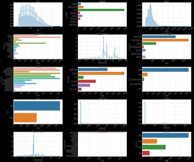
二. 单特征分析
import math
def plot_distribution(dataset, cols, width, height, hspace, wspace):
    fig = plt.figure(figsize = (width, height))
    fig.subplots_adjust(left=None,bottom=None,right=None,top=None,wspace=wspace,hspace=hspace)
    rows = math.ceil(dataset.shape[1] / cols)
    for i,column in enumerate(dataset.columns):
        ax = fig.add_subplot(rows, cols, i+1)
        ax.set_title(column)
        if dataset.dtypes[column] == np.object:
            g = sns.countplot(y=column, data=dataset)
            substrings = [s.get_text()[:18] for s in g.get_yticklabels()]
            g.set(yticklabels = substrings)
            plt.xticks(rotation = 25)
        else:
            g = sns.distplot(dataset[column])
            plt.xticks(rotation = 25)
    plt.tight_layout()
plot_distribution(dataset_raw, cols=3, width=24, height=20, hspace=0.2, wspace=0.5)
# 查看缺失值
import missingno as msno
msno.matrix(dataset_raw, figsize=(16, 5))

# msno.bar(dataset_raw, sort='ascending', figsize=(16,5))

三.数据清洗与特征提取组合
# 创建两个新的数据集
dataset_bin = pd.DataFrame() # 创建离散值数据集
dataset_con = pd.DataFrame() # 创建连续值数据集
- 标签predclass转换
dataset_raw.loc[dataset_raw['predclass']=='<=50K','predclass'] = 0
dataset_raw.loc[dataset_raw['predclass']=='<=50K.','predclass'] = 0
dataset_raw.loc[dataset_raw['predclass']=='>50K','predclass'] = 1
dataset_raw.loc[dataset_raw['predclass']=='>50K.','predclass'] = 1
dataset_bin['predclass'] = dataset_raw['predclass']
dataset_con['predclass'] = dataset_raw['predclass']
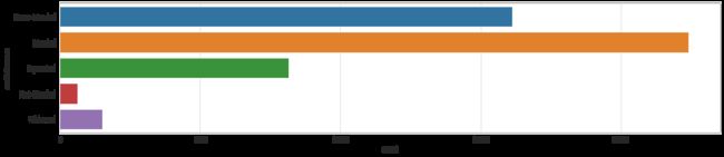
fig = plt.figure(figsize = (20,3))
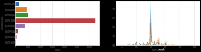
sns.countplot(y = 'predclass', data=dataset_bin)

- Feature: Age
dataset_bin['age'] = pd.cut(dataset_raw['age'], 10) # 将连续值进行切分
dataset_con['age'] = dataset_raw['age']
plt.figure(figsize = (20, 5))
plt.subplot(1, 2, 1)
sns.countplot(y = 'age', data=dataset_bin)
plt.subplot(1, 2, 2)
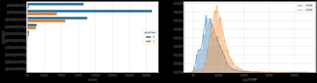
sns.distplot(dataset_con.loc[dataset_con['predclass']==0]['age'], label='<$50K')
sns.distplot(dataset_con.loc[dataset_con['predclass']==1]['age'], label='>$50K')

- Feature: Workclass
dataset_raw.loc[dataset_raw['workclass']=='Without-pay','workclass'] = 'No Pay'
dataset_raw.loc[dataset_raw['workclass']=='Never-worked','workclass'] = 'No Pay'
dataset_raw.loc[dataset_raw['workclass']=='State-gov','workclass'] = 'Gov'
dataset_raw.loc[dataset_raw['workclass']=='Local-gov','workclass'] = 'Gov'
dataset_raw.loc[dataset_raw['workclass']=='Self-emp-not-inc','workclass'] = 'Gov'
dataset_raw.loc[dataset_raw['workclass']=='Federal-gov','workclass'] = 'Self_emp'
dataset_raw.loc[dataset_raw['workclass']=='Self-emp-inc','workclass'] = 'Self_emp'

dataset_bin['workclass'] = dataset_raw['workclass']
dataset_con['workclass'] = dataset_raw['workclass']

plt.figure(figsize = (20,3))
sns.countplot(y = dataset_bin['workclass'])

- Feature: Occupation
dataset_raw.loc[dataset_raw['occupation']=='Adm-clerical', 'occupation'] = 'Managerial'
dataset_raw.loc[dataset_raw['occupation']=='Exec-managerial', 'occupation'] = 'Managerial'
dataset_raw.loc[dataset_raw['occupation']=='Handlers-cleaners', 'occupation'] = 'Technology'
dataset_raw.loc[dataset_raw['occupation']=='Prof-specialty', 'occupation'] = 'Technology'
dataset_raw.loc[dataset_raw['occupation']=='Craft-repair', 'occupation'] = 'Technology'
dataset_raw.loc[dataset_raw['occupation']=='Tech-support', 'occupation'] = 'Technology'
dataset_raw.loc[dataset_raw['occupation']=='Sales', 'occupation'] = 'Labour'
dataset_raw.loc[dataset_raw['occupation']=='Transport-moving', 'occupation'] = 'Labour'
dataset_raw.loc[dataset_raw['occupation']=='Farming-fishing', 'occupation'] = 'Labour'
dataset_raw.loc[dataset_raw['occupation']=='Machine-op-inspct', 'occupation'] = 'Labour'
dataset_raw.loc[dataset_raw['occupation']=='Protective-serv', 'occupation'] = 'Force'
dataset_raw.loc[dataset_raw['occupation']=='Armed-Forces', 'occupation'] = 'Force'
dataset_raw.loc[dataset_raw['occupation']=='Priv-house-serv', 'occupation'] = 'Service'
dataset_raw.loc[dataset_raw['occupation']=='Other-service', 'occupation'] = 'Service'

dataset_bin['occupation'] = dataset_con['occupation'] = dataset_raw['occupation']

plt.figure(figsize = (20,4))
sns.countplot(y = dataset_bin['occupation'])

- Feature: Native Country
def country_apply(data):
    if data['native-country'] == 'United-States':
        return 'USA'
    elif data['native-country'] in ['China','Hong','Taiwan']:
        return 'China'
    elif data['native-country'] in ['Canada','Portugal','France','Outlying-US(Guam-USVI-etc)','South'
                                    'Yugoslavia','England','Germany','Greece','Scotland','Italy',
                                    'Ireland','Poland','Hungary', 'Holand-Netherlands','Japan']:
        return 'Developed_country'
    else:
        return 'Developing_country'
dataset_bin['country'] = dataset_raw.apply(country_apply, axis='columns')
dataset_con['country'] = dataset_raw.apply(country_apply, axis='columns')

plt.figure(figsize = (20, 4))
sns.countplot(y = dataset_bin['country'])

- Feature: Education
dataset_raw.loc[dataset_raw['education']=='Preschool', 'education'] = 'Pre-6th'
dataset_raw.loc[dataset_raw['education']=='1st-4th', 'education'] = 'Pre-6th'
dataset_raw.loc[dataset_raw['education']=='5th-6th', 'education'] = 'Pre-6th'
dataset_raw.loc[dataset_raw['education']=='7th-8th', 'education'] = '7th-12th'
dataset_raw.loc[dataset_raw['education']=='9th', 'education'] = '7th-12th'
dataset_raw.loc[dataset_raw['education']=='10th', 'education'] = '7th-12th'
dataset_raw.loc[dataset_raw['education']=='11th', 'education'] = '7th-12th'
dataset_raw.loc[dataset_raw['education']=='12th', 'education'] = '7th-12th'
dataset_raw.loc[dataset_raw['education']=='Masters', 'education'] = 'Postgraduate'
dataset_raw.loc[dataset_raw['education']=='Doctorate', 'education'] = 'Postgraduate'
dataset_raw.loc[dataset_raw['education']=='Prof-school', 'education'] = 'Postgraduate'
dataset_raw.loc[dataset_raw['education']=='Assoc-acdm', 'education'] = 'Associate'
dataset_raw.loc[dataset_raw['education']=='Assoc-voc', 'education'] = 'Associate'

dataset_bin['education'] = dataset_raw['education']
dataset_con['education'] = dataset_raw['education']

plt.figure(figsize = (20,4))
sns.countplot(y = dataset_bin['education'])

- Feature: Marital Status
dataset_raw.loc[dataset_raw['marital-status'] == 'Never-married'        , 'marital-status'] = 'Never-Married'
dataset_raw.loc[dataset_raw['marital-status'] == 'Married-AF-spouse'    , 'marital-status'] = 'Married'
dataset_raw.loc[dataset_raw['marital-status'] == 'Married-civ-spouse'   , 'marital-status'] = 'Married'
dataset_raw.loc[dataset_raw['marital-status'] == 'Married-spouse-absent', 'marital-status'] = 'Not-Married'
dataset_raw.loc[dataset_raw['marital-status'] == 'Separated'            , 'marital-status'] = 'Separated'
dataset_raw.loc[dataset_raw['marital-status'] == 'Divorced'             , 'marital-status'] = 'Separated'
dataset_raw.loc[dataset_raw['marital-status'] == 'Widowed'              , 'marital-status'] = 'Widowed'

dataset_bin['marital-status'] = dataset_raw['marital-status']
dataset_con['marital-status'] = dataset_raw['marital-status']

plt.figure(figsize = (20,4))
sns.countplot(y = dataset_bin['marital-status'])
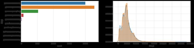
- Feature: Final Weight
dataset_bin['fnlwgt'] = pd.cut(dataset_raw['fnlwgt'], 10)
dataset_con['fnlwgt'] = dataset_raw['fnlwgt']

plt.figure(figsize = (20, 5))
plt.subplot(1, 2, 1)
sns.countplot(y = 'fnlwgt', data=dataset_bin)
plt.subplot(1, 2, 2)
sns.distplot(dataset_con.loc[dataset_con['predclass']==0]['fnlwgt'], label='<$50K')
sns.distplot(dataset_con.loc[dataset_con['predclass']==1]['fnlwgt'], label='>$50K')
- Feature: Education Number
dataset_bin['education-num'] = pd.cut(dataset_raw['education-num'], 8)
dataset_con['education-num'] = dataset_raw['education-num']

plt.figure(figsize = (20, 5))
plt.subplot(1, 2, 1)
sns.countplot(y = 'education-num', data=dataset_bin)
plt.subplot(1, 2, 2)
sns.distplot(dataset_con.loc[dataset_con['predclass']==0]['education-num'], label='<$50K')
sns.distplot(dataset_con.loc[dataset_con['predclass']==1]['education-num'], label='>$50K')
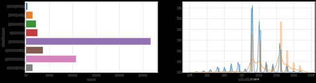
- Feature: Hours per Week
dataset_bin['hours-per-week'] = pd.cut(dataset_raw['hours-per-week'], 8)
dataset_con['hours-per-week'] = dataset_raw['hours-per-week']

plt.figure(figsize = (20, 5))
plt.subplot(1, 2, 1)
sns.countplot(y = 'hours-per-week', data=dataset_bin)
plt.subplot(1, 2, 2)
sns.distplot(dataset_con.loc[dataset_con['predclass']==0]['hours-per-week'], label='<$50K')
sns.distplot(dataset_con.loc[dataset_con['predclass']==1]['hours-per-week'], label='>$50K')
- Feature: Capital Gain
- Feature: Capital Loss
- Features: Race, Sex, Relationship
# 这些就直接用了
dataset_con['sex'] = dataset_bin['sex'] = dataset_raw['sex']
dataset_con['race'] = dataset_bin['race'] = dataset_raw['race']
dataset_con['relationship'] = dataset_bin['relationship'] = dataset_raw['relationship']
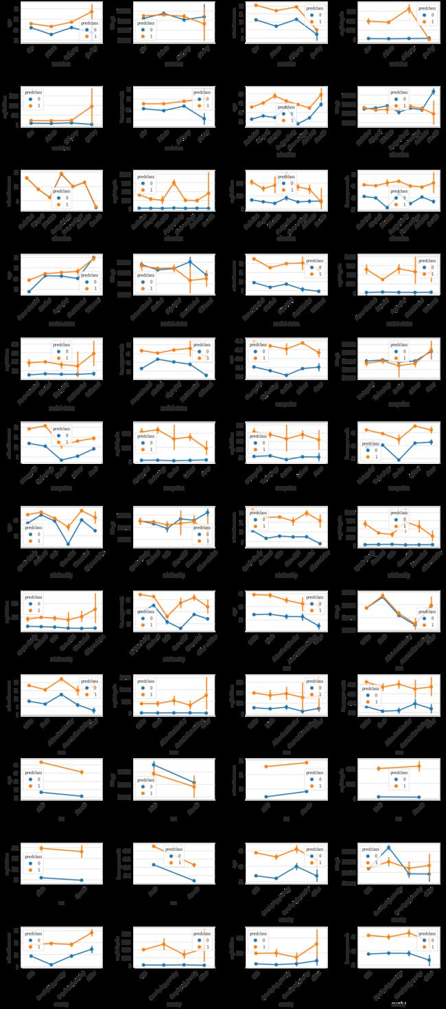
四. 多变量之间的关系
def plot_bivariate_bar(data, hue, cols, width, height, hspace, wspace):
#     data = data.select_dtypes(include = [np.object])
    fig = plt.figure(figsize = (width, height))
    fig.subplots_adjust(left=None,right=None,top=None,bottom=None,wspace=wspace,hspace=hspace)
    rows = math.ceil((data.shape[1]) / cols)
    for i,column in enumerate(data.columns):
        ax = fig.add_subplot(rows, cols, i+1)
        ax.set_title(column)
        if data.dtypes[column] == np.object:
            g = sns.countplot(y=column, hue=hue, data=data)
            substrings = [s.get_text()[:10] for s in g.get_yticklabels()]
            g.set(yticklabels=substrings)
        else:
            g = sns.distplot(data[column])
            plt.xticks(rotation = 25)
plot_bivariate_bar(dataset_con,hue='predclass',cols=3,width=24,height=20,hspace=0.4,wspace=0.2)

obj_list = ['workclass','education','marital-status','occupation','relationship','race','sex','country']
int_list = ['age','fnlwgt','education-num','capital-gain','capital-loss','hours-per-week']

plt.figure(figsize = (16,36))
i = 1
for o in obj_list:
    for t in int_list:
        plt.subplot(12,4,i)
        sns.pointplot(x=o, y=t, hue='predclass', data=dataset_con)
        plt.xticks(rotation=45)
        i += 1
plt.tight_layout()
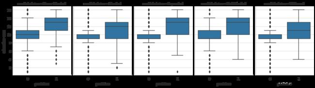
# 婚姻状况和教育对收入的影响
g = sns.FacetGrid(dataset_con, col='marital-status', height=4, aspect=0.7)
g.map(sns.boxplot, 'predclass', 'education-num')
plt.figure(figsize = (20, 5))
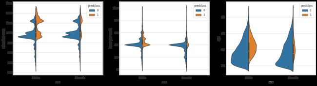
# 性别、教育对收入的影响
plt.subplot(1,3,1)
sns.violinplot(x='sex',y='education-num',hue='predclass',data=dataset_con,split=True,scale='count')
# 性别、工作时长对收入的影响
plt.subplot(1,3,2)
sns.violinplot(x='sex',y='hours-per-week',hue='predclass',data=dataset_con,split=True,scale='count')
# 性别、年龄对收入的影响
plt.subplot(1,3,3)
sns.violinplot(x='sex',y='age',hue='predclass',data=dataset_con,split=True,scale='count')
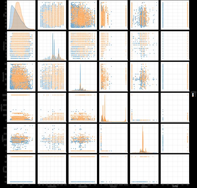
# 不同特征之间的散点图分布
sns.pairplot(dataset_con[['age','education-num','hours-per-week','capital-gain','capital-loss','predclass']],
            hue='predclass', diag_kind='kde', height=4)
五. 创造新的特征
# 年龄和工作时长
dataset_con['age-hours'] = dataset_con['age'] * dataset_con['hours-per-week']
dataset_bin['age-hours'] = pd.cut(dataset_con['age-hours'], 10)

plt.figure(figsize = (20,5))
plt.subplot(1, 2, 1)
sns.countplot(y = 'age-hours', hue='predclass', data=dataset_bin)
plt.subplot(1, 2, 2)
sns.distplot(dataset_con.loc[dataset_con['predclass']==0]['age-hours'],label='<$50K')
sns.distplot(dataset_con.loc[dataset_con['predclass']==1]['age-hours'],label='>$50K')
plt.legend()
# 性别和婚姻
dataset_bin['sex-marital']=dataset_con['sex-marital']=dataset_con['sex']+dataset_con['marital-status']

plt.figure(figsize = (20, 5))
sns.countplot(y='sex-marital', hue='predclass', data=dataset_bin)

未完待续…