SITF特征原理描述及其匹配处理（一）

自1977年Moravec提出Moravec角点检测算子，接下来的一段时间内，就有各种改进的角点检测算子，如Harris角点检测算子、Shi-Tomasi角点检测算子，但是这些都是单维度的角点，直到1999年David G.Lowe提出了一种基于尺度空间的，对图像缩放、旋转、甚至仿射变换保持不变性的图像局部特征描述算子——SIFT（尺度不变特征变换），用多维向量来描述一个特征点，是过去十年中最成功的图像据不描述子之一。

SITF特征原理描述

1.SIFT是什么

SIFT特征提取算法的实质是在不同的尺度空间上查找关键点（特征点），计算关键点的大小、方向、尺度信息，利用这些信息组成关键点对特征点进行描述的问题。SIFT的不变形体现在：尺度、方向、位移和光照。它所查找的关键点都是一些十分突出，不会因光照，仿射便函和噪声等因素而变换的“稳定”特征点，如角点、边缘点、暗区的亮点以及亮区的暗点等。

2.SIFT的流程

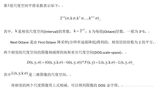
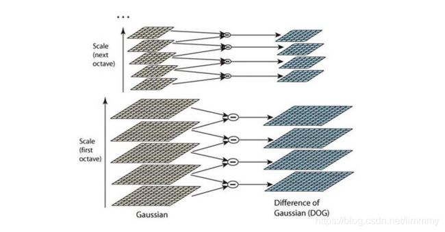
2.1构建尺度空间和高斯差分金字塔

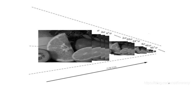
SIFT算法在多尺度空间进行特征点的检测和提取，保证了特征具有尺度不变性。尺度空间理论目的的是模拟图像数据的多尺度特征，通过输入的图像和不同的高斯核作卷积得到的二维图像的高斯尺度空间：

其中，是尺度空间因子σ，其大小决定图像的平滑程度，大尺度对应图像的概貌特征，小尺度对应图像的细节特征。*代表卷积，F(x,y)是输入图像，G(x,y,σ)是尺度可变高斯函数：

二维图像的尺度空间图像如下：

2.1 空间极值点初步检测

为了计算尺度空间极值点，需要将尺度空间上的每一个像素点与其3×3邻域的和这一像素点相邻的８个点及上下两层金字塔相对应的9×2共26个相邻点进行一一比较，只有当这个点是这26个点中的最大点或者最小点时，如此可以保证检测到的关键点在尺度空间和二维图像空间上都是局部极值点。

利用上述方法检测出的候选极值点中包含很多低对比度的点和部分 DOG算子产生的边缘响应点，需要进行过滤以精确特征点的位置，提高SIFT算法的抗噪性。于是需要下一步稳定关键点的精确定位。

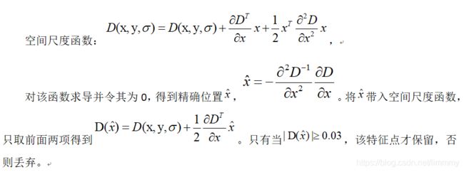
2.2 稳定关键点的精确定位

在已经检测到的特征点中要去掉低对比度的特征点和不稳定的边缘响应点。

去除对比度低的特征点

去除不稳定的边缘响应点

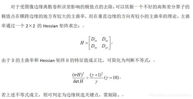
2.4 稳定关键点方向信息分配

稳定的极值点是在不同尺度空间下提取的，这保证了关键点的尺度不变性。为关键点分配方向信息所要解决的问题是使得关键点对图像角度和旋转具有不变性。方向的分配是通过求每个极值点的梯度来实现的。对于任一关键点，其梯度模值表述为：
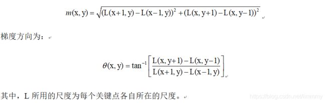至此，图像的关键点以检测完毕，每个关键点有三个信息：位置、所处尺度、方向。由此可以确定一个SIFT特征区域。利用关键点邻域像素的梯度方向分布特性为每个关键点指定方向参数，使算子具备旋转不变性。

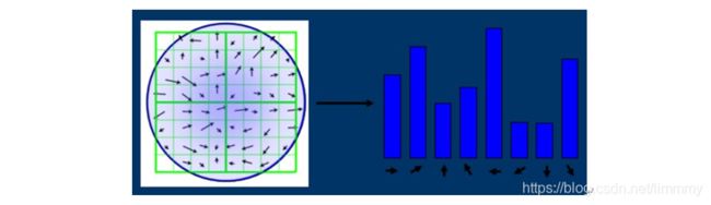
按照梯度方向直方图的方式分配关键点的方向：以关键点为中心的领域窗口内采样，并用直方图统计邻域像素的梯度方向。梯度直方图的范围是0～360度，其中每10度一个柱，总共36个柱。随着距中心点越远的邻域其对直方图的贡献也响应减小。Lowe论文中还提到要使用高斯函数对直方图进行平滑，减少突变的影响。

2.5 关键点描述

在以关键点为中心的邻域窗口内采样，并用直方图统计邻域像素的梯度方向。直方图的峰值则代表了该特征点处邻域梯度的主方向，将坐标轴旋转为关键点的方向，以确保旋转不变性。通过确定关键点邻域所在尺度空间的16×16像素大小的邻域，再将此邻域均匀地分为4×4个窗口，对每个窗口计算8个方向分量值，根据位置依次排序，得到128维的SIFT 特征向量。将这个向量归一化之后，就进一步去除了光照的影响。

David G.Lowed的实验结果表明：对每个关键点，采用448共128维向量的描述子进项关键点表征，综合效果最佳：

一个4×4的计算出一个直方图，每个直方图有8个方向，4×4×8=128维

在求出4 * 4 * 8的128维特征向量后，此时SIFT特征向量已经去除了尺度变化、旋转等几何变形因素的影响。而图像的对比度变化相当于每个像素点乘上一个因子，光照变化是每个像素点加上一个值，但这些对图像归一化的梯度没有影响。因此将特征向量的长度归一化，则可以进一步去除光照变化的影响。

对于一些非线性的光照变化，SIFT并不具备不变性，但由于这类变化影响的主要是梯度的幅值变化，对梯度的方向影响较小，因此作者通过限制梯度幅值的值来减少这类变化造成的影响。

2.2 特征点匹配

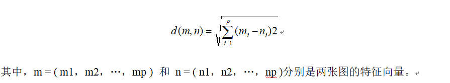
特征点的匹配是通过计算两组特征点的128维的关键点的欧式距离实现的。欧式距离越小，则相似度越高，当欧式距离小于设定的阈值时，可以判定为匹配成功。欧式距离的公式为：
选择SIFT算法进行分析，是因为该算法不但对于旋转、尺度缩放、亮度变化保持不变性，而且对视角变化、仿射变换、噪声也保持一定程度的稳定性。且该方法对特征点的个数和有效点的比例没有要求。当特征点不是很多时，经优化的SIFT匹配算法甚至可以达到实时的要求。而且可以很方便的与其他形式的特征向量进行联合。

3.SIFT与Harris的匹配效果比对

根据SIFT可以解决的问题
• 目标的旋转、缩放、平移（RST）
• 图像仿射/投影变换（视点viewpoint）
• 弱光照影响（illumination）
• 部分目标遮挡（occlusion）
• 杂物场景（clutter）
• 噪声

我选择了几组图像与Harris的处理结果进行比对
Ps:彩色的是SIFT效果，黑白的是HARRIS，下面不做备注了

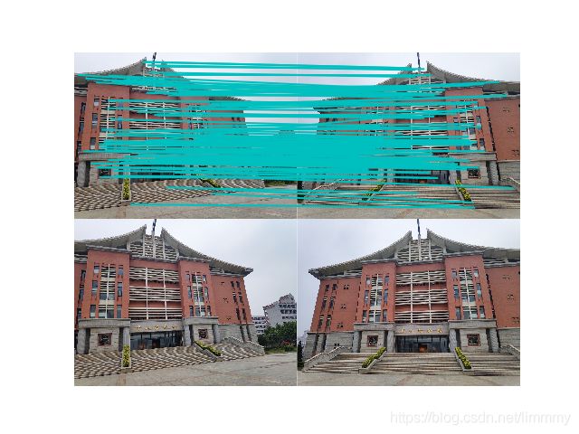
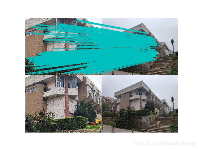
（1）第一组（弱光照且图片纹理相似）

SIFT特征匹配处理效果

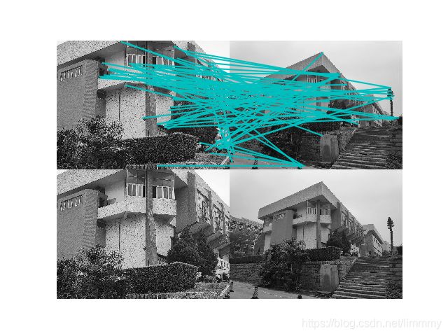
Harris特征匹配处理效果

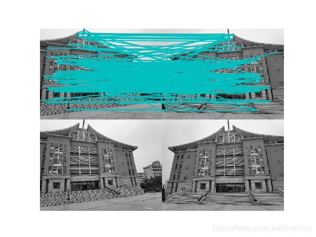
实验结果及其分析：第一组图像的特征是光线较弱且建筑物纹理较相似
Harris找到的特征点明显多于SIFT找到的，而且因为我选择比对的两张原图拍摄角度近似水平的，所以特征点相连的线应该是平行线结果才比较准确，Harris的图像可以看出有交叉线，那几条连线明显属于错误匹配的。
说明:在弱光线的情况下，SIFT的匹配效果优于Harris

（2）第二组（旋转）

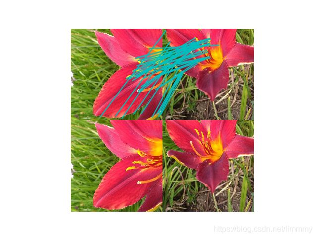
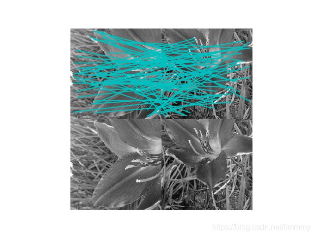
实验结果及其分析：第二组图像的特征是两张图片旋转一定角度
SIFT找到的关键点大都是花瓣的边缘（角点）或者花蕊（颜色较周围差异较大的点），Harris在草的部分也标注为关键点并进行匹配，效果不准确，那些点是无效点。
说明：在旋转（一定的角度，太大可能也匹配不出来，还没测试过）的情况下，SIFT的匹配效果优于Harris

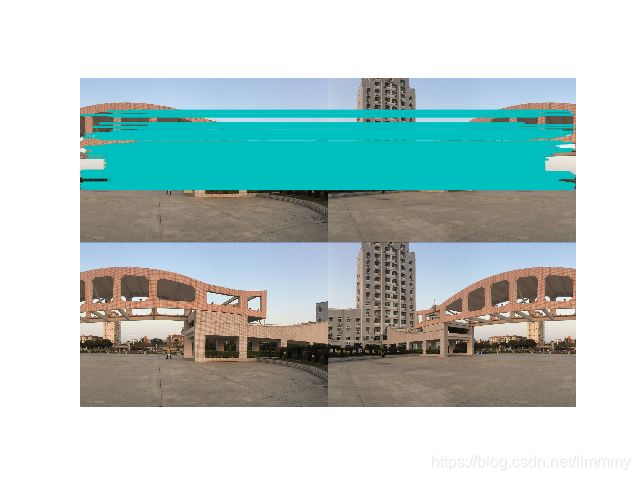
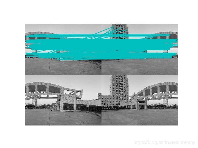
（3）第三组（缩放）

实验结果及其分析：第三组图像的特征是同一建筑物同一视角，镜头远近不同（图片的缩放）
第一张图较近，第二张图较远，所以SIFT的连接线呈现的形状符合规律，Harris则杂乱无章。
说明：在缩放的情况下，SIFT的匹配效果优于Harris

（4）第四组（平移）

实验结果及其分析：第四组图像的特征是平移镜头的建筑物
SIFT和Harris找到的关键点大都准确且连线都近乎平行，处了Harris有几条匹配错误。
说明：在平移的情况下，SIFT的匹配效果与Harris相近。

（5）运行时间的比对

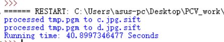
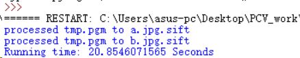
sift运行时间：

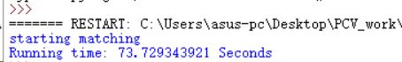
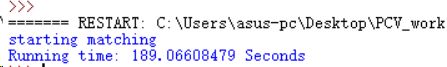
Harris运行时间：

sift运行时间：

Harris运行时间：

实验结果及其分析：
SIFT的总运行时间总是少于Harris的。
原因应该在找特征点上以及特征点的匹配上。Harris总是找到一些不稳定点，匹配的时候时间花费的也比较多。

总结

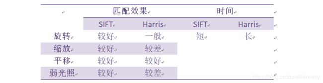
就上面几种情况来说，SIFT是优于Harris的。其他的情况还未测试。

以下是Harris.py的代码

# -*- coding: utf-8 -*-
from pylab import *
from numpy import *
from PIL import Image
from scipy.ndimage import filters
from PCV.tools.imtools import imresize

import time

#harris.py

#返回像素值为Harris响应函数值的一幅图像
def compute_harris_response(im,sigma=3):
    """ Compute the Harris corner detector response function 
        for each pixel in a graylevel image. """
    
    # derivatives 计算导数
    imx = zeros(im.shape)
    filters.gaussian_filter(im, (sigma,sigma), (0,1), imx)
    imy = zeros(im.shape)
    filters.gaussian_filter(im, (sigma,sigma), (1,0), imy)
    
    # compute components of the Harris matrix  计算Harris矩阵的分量
    Wxx = filters.gaussian_filter(imx*imx,sigma)
    Wxy = filters.gaussian_filter(imx*imy,sigma)
    Wyy = filters.gaussian_filter(imy*imy,sigma)
    
    # determinant and trace  计算特征值和迹
    Wdet = Wxx*Wyy - Wxy**2
    Wtr = Wxx + Wyy
    
    return Wdet / Wtr
   
#从Harris响应图像中返回角点  
def get_harris_points(harrisim,min_dist=10,threshold=0.1):
    """ Return corners from a Harris response image
        min_dist is the minimum number of pixels separating 
        corners and image boundary. """
    
    # find top corner candidates above a threshold 高于阈值的候选角点
    corner_threshold = harrisim.max() * threshold
    harrisim_t = (harrisim > corner_threshold) * 1
    
    # get coordinates of candidates 得到候选坐标
    coords = array(harrisim_t.nonzero()).T
    
    # ...and their values 以及他们的响应值
    candidate_values = [harrisim[c[0],c[1]] for c in coords]
    
    # sort candidates (reverse to get descending order)对候选点按照Harris响应值进行排序
    index = argsort(candidate_values)[::-1]
    
    # store allowed point locations in array将可行点保存数组
    allowed_locations = zeros(harrisim.shape)
    allowed_locations[min_dist:-min_dist,min_dist:-min_dist] = 1
    
    # select the best points taking min_distance into account按照min_distance原则，选择最佳Harris点
    filtered_coords = []
    for i in index:
        if allowed_locations[coords[i,0],coords[i,1]] == 1:
            filtered_coords.append(coords[i])
            allowed_locations[(coords[i,0]-min_dist):(coords[i,0]+min_dist), 
                        (coords[i,1]-min_dist):(coords[i,1]+min_dist)] = 0
    
    return filtered_coords
    
#绘制图像中检测到的角点   
def plot_harris_points(image,filtered_coords):
    """ Plots corners found in image. """
    
    figure()
    gray()
    imshow(image)
    plot([p[1] for p in filtered_coords],
                [p[0] for p in filtered_coords],'*')
    axis('off')
    show()
   
#返回点周围2*wid+1个像素的值（假设选组点的min_distance>wid）
def get_descriptors(image,filtered_coords,wid=5):
    """ For each point return pixel values around the point
        using a neighbourhood of width 2*wid+1. (Assume points are 
        extracted with min_distance > wid). """
    
    desc = []
    for coords in filtered_coords:
        patch = image[coords[0]-wid:coords[0]+wid+1,
                            coords[1]-wid:coords[1]+wid+1].flatten()
        desc.append(patch)
    
    return desc

#对于第一幅图像中的每个角点描述子，使用归一化互相关，选取他在第二幅图像中的匹配角点
def match(desc1,desc2,threshold=0.5):
    """ For each corner point descriptor in the first image, 
        select its match to second image using
        normalized cross correlation. """
    
    n = len(desc1[0])
    
    # pair-wise distances
    d = -ones((len(desc1),len(desc2)))
    for i in range(len(desc1)):
        for j in range(len(desc2)):
            d1 = (desc1[i] - mean(desc1[i])) / std(desc1[i])
            d2 = (desc2[j] - mean(desc2[j])) / std(desc2[j])
            ncc_value = sum(d1 * d2) / (n-1) 
            if ncc_value > threshold:
                d[i,j] = ncc_value
            
    ndx = argsort(-d)
    matchscores = ndx[:,0]
    
    return matchscores

#从第二幅向第一幅图像匹配，然后过滤掉两种方法中都是最好的匹配
def match_twosided(desc1,desc2,threshold=0.5):
    """ Two-sided symmetric version of match(). """
    
    matches_12 = match(desc1,desc2,threshold)
    matches_21 = match(desc2,desc1,threshold)
    
    ndx_12 = where(matches_12 >= 0)[0]
    
    # remove matches that are not symmetric去除非对称匹配
    for n in ndx_12:
        if matches_21[matches_12[n]] != n:
            matches_12[n] = -1
    
    return matches_12

#分别在两边绘制出图像，使用线段链接匹的像素点可视化
def appendimages(im1,im2):
    """ Return a new image that appends the two images side-by-side. """
    
    # select the image with the fewest rows and fill in enough empty rows
    rows1 = im1.shape[0]    
    rows2 = im2.shape[0]
    
    if rows1 < rows2:
        im1 = concatenate((im1,zeros((rows2-rows1,im1.shape[1]))),axis=0)
    elif rows1 > rows2:
        im2 = concatenate((im2,zeros((rows1-rows2,im2.shape[1]))),axis=0)
    # if none of these cases they are equal, no filling needed.
    
    return concatenate((im1,im2), axis=1)
    
def plot_matches(im1,im2,locs1,locs2,matchscores,show_below=True):
    """ Show a figure with lines joining the accepted matches 
        input: im1,im2 (images as arrays), locs1,locs2 (feature locations), 
        matchscores (as output from 'match()'), 
        show_below (if images should be shown below matches). """
    
    im3 = appendimages(im1,im2)
    if show_below:
        im3 = vstack((im3,im3))
    
    imshow(im3)
    
    cols1 = im1.shape[1]
    for i,m in enumerate(matchscores):
        if m>0:
            plot([locs1[i][1],locs2[m][1]+cols1],[locs1[i][0],locs2[m][0]],'c')
    axis('off')

start=time.clock()

im1 = array(Image.open("a.jpg").convert("L"))
im2 = array(Image.open("b.jpg").convert("L"))
# resize to make matching faster
im1 = imresize(im1,(im1.shape[1]/2,im1.shape[0]/2))
im2 = imresize(im2,(im2.shape[1]/2,im2.shape[0]/2))

wid = 5
harrisim = compute_harris_response(im1,5) 
filtered_coords1 = get_harris_points(harrisim,wid+1) 
d1 = get_descriptors(im1,filtered_coords1,wid)

harrisim = compute_harris_response(im2,5) 
filtered_coords2 = get_harris_points(harrisim,wid+1) 
d2 = get_descriptors(im2,filtered_coords2,wid)

print 'starting matching'
matches = match_twosided(d1,d2)

figure()
gray() 
plot_matches(im1,im2,filtered_coords1,filtered_coords2,matches) 
show()


end = time.clock()
print('Running time: %s Seconds'%(end-start))

以下是SIFT.py的代码

from pylab import *
from numpy import *
from PIL import Image
from PCV.localdescriptors import sift

from PIL import Image
from numpy import *
from pylab import *
import os

def process_image(imagename,resultname,params="--edge-thresh 10 --peak-thresh 5"):
    """ Process an image and save the results in a file. """

    if imagename[-3:] != 'pgm':
        # create a pgm file
        im = Image.open(imagename).convert('L')
        im.save('tmp.pgm')
        imagename = 'tmp.pgm'

    cmmd = str("C:\\Users\\asus-pc\\Desktop\\PCV_work\\win64vlfeat\\sift.exe "+imagename+" --output="+resultname+
                " "+params)
    os.system(cmmd)
    print 'processed', imagename, 'to', resultname


def read_features_from_file(filename):
    """ Read feature properties and return in matrix form. """
    
    f = loadtxt(filename)
    return f[:,:4],f[:,4:] # feature locations, descriptors


def write_features_to_file(filename,locs,desc):
    """ Save feature location and descriptor to file. """
    savetxt(filename,hstack((locs,desc)))
    

def plot_features(im,locs,circle=False):
    """ Show image with features. input: im (image as array), 
        locs (row, col, scale, orientation of each feature). """

    def draw_circle(c,r):
        t = arange(0,1.01,.01)*2*pi
        x = r*cos(t) + c[0]
        y = r*sin(t) + c[1]
        plot(x,y,'b',linewidth=2)

    imshow(im)
    if circle:
        for p in locs:
            draw_circle(p[:2],p[2]) 
    else:
        plot(locs[:,0],locs[:,1],'ob')
    axis('off')


def match(desc1,desc2):
    """ For each descriptor in the first image, 
        select its match in the second image.
        input: desc1 (descriptors for the first image), 
        desc2 (same for second image). """
    
    desc1 = array([d/linalg.norm(d) for d in desc1])
    desc2 = array([d/linalg.norm(d) for d in desc2])
    
    dist_ratio = 0.6
    desc1_size = desc1.shape
    
    matchscores = zeros((desc1_size[0]),'int')
    desc2t = desc2.T # precompute matrix transpose
    for i in range(desc1_size[0]):
        dotprods = dot(desc1[i,:],desc2t) # vector of dot products
        dotprods = 0.9999*dotprods
        # inverse cosine and sort, return index for features in second image
        indx = argsort(arccos(dotprods))
        
        # check if nearest neighbor has angle less than dist_ratio times 2nd
        if arccos(dotprods)[indx[0]] < dist_ratio * arccos(dotprods)[indx[1]]:
            matchscores[i] = int(indx[0])
    
    return matchscores


def appendimages(im1,im2):
    """ Return a new image that appends the two images side-by-side. """
    
    # select the image with the fewest rows and fill in enough empty rows
    rows1 = im1.shape[0]    
    rows2 = im2.shape[0]
    
    if rows1 < rows2:
        im1 = concatenate((im1,zeros((rows2-rows1,im1.shape[1]))), axis=0)
    elif rows1 > rows2:
        im2 = concatenate((im2,zeros((rows1-rows2,im2.shape[1]))), axis=0)
    # if none of these cases they are equal, no filling needed.
    
    return concatenate((im1,im2), axis=1)


def plot_matches(im1,im2,locs1,locs2,matchscores,show_below=True):
    """ Show a figure with lines joining the accepted matches
        input: im1,im2 (images as arrays), locs1,locs2 (location of features), 
        matchscores (as output from 'match'), show_below (if images should be shown below). """
    
    im3 = appendimages(im1,im2)
    if show_below:
        im3 = vstack((im3,im3))
    
    # show image
    imshow(im3)
    
    # draw lines for matches
    cols1 = im1.shape[1]
    for i,m in enumerate(matchscores):
        if m>0:
            plot([locs1[i][0],locs2[m][0]+cols1],[locs1[i][1],locs2[m][1]],'c')
    axis('off')


def match_twosided(desc1,desc2):
    """ Two-sided symmetric version of match(). """
    
    matches_12 = match(desc1,desc2)
    matches_21 = match(desc2,desc1)
    
    ndx_12 = matches_12.nonzero()[0]
    
    # remove matches that are not symmetric
    for n in ndx_12:
        if matches_21[int(matches_12[n])] != n:
            matches_12[n] = 0
    
    return matches_12

import time
start =time.clock()

imname1 = 'a.jpg'
imname2 = 'b.jpg'

# process and save features to file
process_image(imname1, imname1+'.sift')
process_image(imname2, imname2+'.sift')

# read features and match
l1,d1 = read_features_from_file(imname1+'.sift')
l2,d2 = read_features_from_file(imname2+'.sift')
matchscores = match_twosided(d1, d2)

# load images and plot
im1 = array(Image.open(imname1))
im2 = array(Image.open(imname2))

plot_matches(im1,im2,l1,l2,matchscores,show_below=True)
show()

end = time.clock()
print('Running time: %s Seconds'%(end-start))