An Introduction to Greta

I was surprised by greta. I had assumed that the tensorflow and reticulate packages would eventually enable R developers to look beyond deep learning applications and exploit the TensorFlow platform to create all manner of production-grade statistical applications. But I wasn’t thinking Bayesian. After all, Stan is probably everything a Bayesian modeler could want. Stan is a powerful, production-level probability distribution modeling engine with a slick R interface, deep documentation, and a dedicated development team.

But greta lets users write TensorFlow-based Bayesian models directly in R! What could be more charming? greta removes the barrier of learning an intermediate modeling language while still promising to deliver high-performance MCMC models that run anywhere TensorFlow can go.

In this post, I’ll introduce you to greta with a simple model used by Richard McElreath in section 8.3 of his iconoclastic book:Statistical Rethinking: A Bayesian Course with Examples in R and Stan. This model seeks to explain the log of a country’s GDP based on a measure of terrain ruggedness while controlling for whether or not the country is in Africa. I am going to use it just to illustrate MCMC sampling with greta. The extended example in McElreath’s book, however, is a meditation on the subtleties of modeling interactions, and is well worth studying.

First, we load the required packages and fetch the data. DiagrammeR is for plotting the TensorFlow flow diagram of the model, andbayesplot is used to plot trace diagrams of the Markov chains. The rugged data set which provides 52 variables for 234 is fairly interesting, but we will use a trimmed-down data set with only 170 counties and three variables.

library(rethinking)
library(greta)
library(DiagrammeR)
library(bayesplot)
library(ggplot2) # Example from section 8.3 Statistical Rethinking data(rugged) d <- rugged d$log_gdp <- log(d$rgdppc_2000) dd <- d[complete.cases(d$rgdppc_2000), ] dd_trim <- dd[ , c("log_gdp","rugged","cont_africa")] head(dd_trim)

##     log_gdp rugged cont_africa
## 3  7.492609  0.858           1
## 5  8.216929  3.427           0
## 8  9.933263  0.769           0
## 9  9.407032  0.775           0
## 10 7.792343  2.688           0
## 12 9.212541  0.006           0

set.seed(1234)

In this section of code, we set up the TensorFlow data structures. The first step is to move the data into greta arrays. These data structures behave similarly to R arrays in that they can be manipulated with functions. However, greta doesn’t immediately calculate values for new arrays. It works out the size and shape of the result and creates a place-holder data structure.

#data
g_log_gdp <- as_data(dd_trim$log_gdp)
g_rugged <- as_data(dd_trim$rugged)
g_cont_africa <- as_data(dd_trim$cont_africa)

In this section, we set up the Bayesian model. All parameters need prior probability distributions. Note that the parameters a, bR,bA, bAR, sigma, and mu are all new greta arrays that don’t contain any data. a is 1 x 1 array and mu is a 170 x 1 array with one slot for each observation.

The distribution() function sets up the likelihood function for the model.

# Variables and Priors

a <- normal(0, 100)
bR <- normal(0, 10) bA <- normal(0, 10) bAR <- normal(0,10) sigma <- cauchy(0,2,truncation=c(0,Inf)) a # Look at this greata array

## greta array (variable following a normal distribution)
## 
##      [,1]
## [1,]  ?

# operations
mu <- a + bR*g_rugged + bA*g_cont_africa + bAR*g_rugged*g_cont_africa

dim(mu)

## [1] 170   1

# likelihood
distribution(g_log_gdp) = normal(mu, sigma)

The model() function does all of the work. It fits the model and produces a fairly complicated object organized as three lists that contain, respectively, the R6 class, TensorFlow structures, and the various greta data arrays.

# defining the model
mod <- model(a,bR,bA,bAR,sigma)

str(mod,give.attr=FALSE,max.level=1)

## List of 3
##  $ dag                 :Classes 'dag_class', 'R6' 
##   Public:
##     adjacency_matrix: function () 
##     build_dag: function (greta_array_list) 
##     clone: function (deep = FALSE) 
##     compile: TRUE
##     define_gradients: function () 
##     define_joint_density: function () 
##     define_tf: function () 
##     example_parameters: function (flat = TRUE) 
##     find_node_neighbours: function () 
##     get_tf_names: function (types = NULL) 
##     gradients: function (adjusted = TRUE) 
##     initialize: function (target_greta_arrays, tf_float = tf$float32, n_cores = 2L, 
##     log_density: function (adjusted = TRUE) 
##     make_names: function () 
##     n_cores: 4
##     node_list: list
##     node_tf_names: variable_1 distribution_1 data_1 data_2 operation_1 oper ...
##     node_types: variable distribution data data operation operation oper ...
##     parameters_example: list
##     send_parameters: function (parameters, flat = TRUE) 
##     subgraph_membership: function () 
##     target_nodes: list
##     tf_environment: environment
##     tf_float: tensorflow.python.framework.dtypes.DType, python.builtin.object
##     tf_name: function (node) 
##     trace_values: function ()  
##  $ target_greta_arrays :List of 5
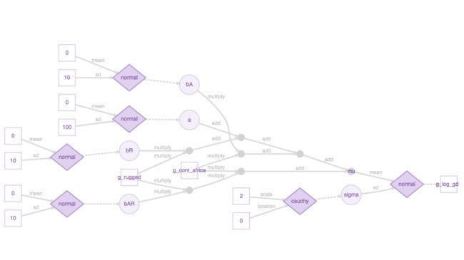
##  $ visible_greta_arrays:List of 9

Plotting mod produces the TensorFlow flow diagram that shows the structure of the underlying TensorFlow model, which is simple for this model and easily interpretable.

# plotting
plot(mod)

Next, we use the greta function mcmc() to sample from the posterior distributions defined in the model.

# sampling
draws <- mcmc(mod, n_samples = 1000)
summary(draws)

## 
## Iterations = 1:1000
## Thinning interval = 1 
## Number of chains = 1 
## Sample size per chain = 1000 
## 
## 1. Empirical mean and standard deviation for each variable,
##    plus standard error of the mean:
## 
##          Mean      SD Naive SE Time-series SE
## a      9.2225 0.13721 0.004339       0.004773
## bR    -0.2009 0.07486 0.002367       0.002746
## bA    -1.9485 0.23033 0.007284       0.004435
## bAR    0.3992 0.13271 0.004197       0.003136
## sigma  0.9527 0.04892 0.001547       0.001744
## 
## 2. Quantiles for each variable:
## 
##          2.5%     25%     50%     75%    97.5%
## a      8.9575  9.1284  9.2306  9.3183  9.47865
## bR    -0.3465 -0.2501 -0.1981 -0.1538 -0.05893
## bA    -2.3910 -2.1096 -1.9420 -1.7876 -1.50781
## bAR    0.1408  0.3054  0.3954  0.4844  0.66000
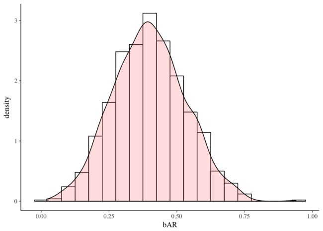
## sigma  0.8616  0.9194  0.9520  0.9845  1.05006

Now that we have the samples of the posterior distributions of the parameters in the model, it is straightforward to examine them. Here, we plot the posterior distribution of the interaction term.

mat <- data.frame(matrix(draws[[1]],ncol=5))
names(mat) <- c("a","bR","bA","bAR","sigma") #head(mat) # http://www.cookbook-r.com/Graphs/Plotting_distributions_(ggplot2)/ ggplot(mat, aes(x=bAR)) + geom_histogram(aes(y=..density..), binwidth=.05, colour="black", fill="white") + geom_density(alpha=.2, fill="#FF6666") 

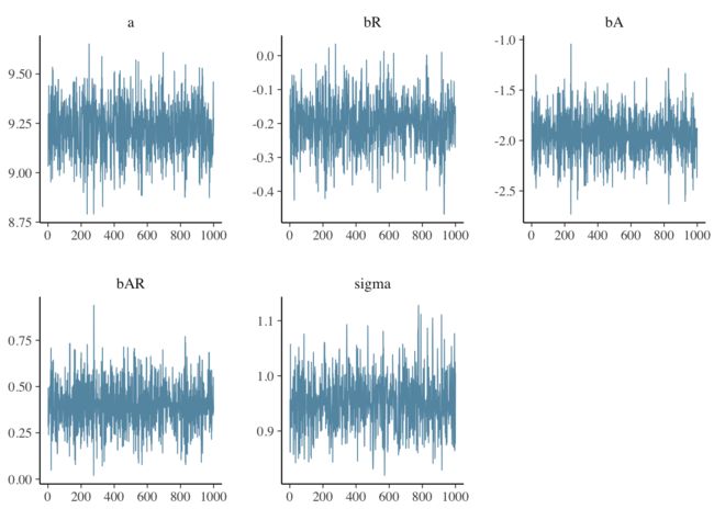
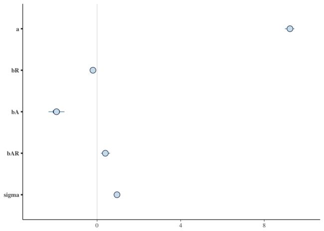
Finally, we examine the trace plots for the MCMC samples using the greta function mcmc_trace(). The plots for each parameter appear to be stationary (flat, i.e., centered on a constant value) and well-mixed (there is no obvious correlation between points).mcmc_intervals() plots the uncertainty intervals for each parameter computed from posterior draws with all chains merged.

mcmc_trace(draws)

mcmc_intervals(draws)

So there it is - a Bayesian model using Hamiltonian Monte Carlo sampling built in R and evaluated by TensorFlow.

For an expert discussion of the model, have a look at McElreath’s book, described at the link above. For more on greta, see thepackage documentation. And please, do take the time to read about greta’s namesake: Greta Hermann, a remarkable woman - mathematician, philosopher, educator, social activist, and theoretical physicist who found the error in John von Neuman’s “proof” of the “No hidden variables theorem” of Quantum Mechanics.

转自：https://rviews.rstudio.com/2018/04/23/on-first-meeting-greta/

转载于:https://www.cnblogs.com/payton/p/8926602.html