SLAM 坐标系变换 (包含CoreSLAM)
1. 基础
- **CoreSLAM(tinySLAM)**主要思想就是基于粒子滤波器(particle filter)将激光数据整合到定位子系统中。
- 目标:算法简单、易于理解、但提供好的性能;且易于集成到基于粒子滤波的框架中。
##1.1 似然函数(Likelihood Function) - 定义:似然函数是一种关于统计模型中的参数的函数,表示模型参数中的似然性。
- 用途:似然函数在统计推断中有重大作用,如在最大似然估计和费雪信息之中的应用等等。
- 概率:用于在已知一些 参 数 \color{red}{参数} 参数的情况下,预测接下来的观测所得到的结果;研究对象为白盒,已知概率分布。
- 似然性:是用于在已知某些观测所得到的结果时,对有关事物的性质的 参 数 \color{red}{参数} 参数进行估计;研究对象为黑盒,概率分布未知。
- 关键特性:似然函数的重要性不是它的具体取值,而是当参数变化时函数到底 变 小 还 是 变 大 \color{red}{变小还是变大} 变小还是变大。对同一个似然函数,如果存在一个参数值,使得它的 函 数 值 达 到 最 大 \color{red}{函数值达到最大} 函数值达到最大的话,那么这个值就是最为“ 合 理 \color{red}{合理} 合理”的参数值。
- 关注目标:关注似然函数的参数,而不是似然函数的值
- a
##1.2 最大似然估计(MLE:Maximum Likelihood Estimation) - 定义:也称为最大概似估计,也叫极大似然估计;是用来估计一个概率模型的参数的一种方法;是一种统计方法,它用来求一个样本集的相关概率密度函数的参数;明确地使用概率模型, 其目标是寻找能够以较高概率产生观察数据的系统发生树。最大似然估计是 似 然 函 数 \color{red}{似然函数} 似然函数最初也是最自然的应用。
- 基本思想:当从模型总体随机抽取n组样本观测值后,最合理的参数估计量应该使得从模型中抽取该 n n n组 样 本 观 测 值 的 概 率 最 大 \color{red}{样本观测值的概率最大} 样本观测值的概率最大,而不是像最小二乘估计法旨在得到使得模型能 最 好 地 拟 合 样 本 数 据 的 参 数 估 计 量 \color{red}{最好地拟合样本数据的参数估计量} 最好地拟合样本数据的参数估计量。
- 合理参数估计:似然函数取得最大值表示相应的参数能够使得统计模型最为合理, 合 理 的 参 数 估 计 量 使 得 样 本 出 现 的 概 率 最 大 \color{red}{合理的参数估计量使得样本出现的概率最大} 合理的参数估计量使得样本出现的概率最大。
- 实现方法:首先选取似然函数(一般是概率密度函数或概率质量函数),整理之后求最大值。实际应用中一般会取似然函数的对数作为求最大值的函数,这样求出的最大值和直接求最大值得到的结果是相同的。
1.2.1 最大似然估计(MLE)与最小二乘法的区别(MLS)
- 最大似然估计:现在已经拿到了很多样本,最大似然估计就是去找到那个(组)参数估计值,使得前面的观测样本发生概率最大。因为你手上的样本已经实现了,其发生概率最大才符合逻辑。这时是求样本所有观测的联合概率最大化,是个连乘积,只要取对数,就变成了线性加总。此时通过对参数求导数,并令一阶导数为零,就可以通过解方程(组),得到最大似然估计值。
- 最小二乘:找到一个(组)估计值,使得实际值与估计值的距离最小,即最好地拟合样本数据。本来用两者差的绝对值汇总并使之最小是最理想的,但绝对值在数学上求最小值比较麻烦,因而替代做法是,找一个(组)估计值,使得实际值与估计值之差的平方加总之后的值最小,称为最小二乘。“二乘”的英文为Least Square,其实英文的字面意思是“平方最小”。这时,将这个差的平方的和式对参数求导数,并取一阶导数为零,就是LSE。
##1.3 布雷森汉姆直线算法(Bresenham’s line algorithm)
- 用途:是用来描绘由两点所决定的直线的算法,它会算出一条线段在n维位图上最接近的点。
- 算法特性:这个算法只会用到较为快速的整数加法、减法和位元移位,常用于绘制电脑画面中的直线。
1.4 蒙特卡罗方法(Monte Carlo method)
- 定义:也称统计模拟方法,是一种以概率统计理论为指导的数值计算方法。是指使用随机数(或更常见的伪随机数)来解决很多计算问题的方法。
- 分类:
- 所求解的问题本身具有内在的随机性,借助计算机的运算能力可以直接模拟这种随机的过程。
- 所求解问题可以转化为某种随机分布的特征数,比如随机事件出现的概率,或者随机变量的期望值。通过随机抽样的方法,以随机事件出现的频率估计其概率,或者以抽样的数字特征估算随机变量的数字特征,并将其作为问题的解。这种方法多用于求解复杂的多维积分问题。
- 基本思想:假设我们要计算一个不规则图形的面积,那么图形的不规则程度和分析性计算(比如,积分)的复杂程度是成正比的。蒙特卡罗方法基于这样的思想:假想你有一袋豆子,把豆子均匀地朝这个图形上撒,然后数这个图形之中有多少颗豆子,这个豆子的数目就是图形的面积。当你的豆子越小,撒的越多的时候,结果就越精确。借助计算机程序可以生成大量均匀分布坐标点,然后统计出图形内的点数,通过它们占总点数的比例和坐标点生成范围的面积就可以求出图形面积。
- 工作流程:
- 第一步:用蒙特卡罗方法模拟某一过程时,需要产生各种 概 率 分 布 的 随 机 变 量 \color{red}{概率分布的随机变量} 概率分布的随机变量
- 第二步:用统计方法把模型的 数 字 特 征 \color{red}{数字特征} 数字特征估计出来,从而得到实际问题的数值解
- 应用:
- 通常蒙特卡罗方法通过构造匹配一定规则的随机数来解决数学上的各种问题。对于那些由于计算过于复杂而难以得到解析解或者根本没有解析解的问题,蒙特卡罗方法是一种有效的求出数值解的方法。一般蒙特卡罗方法在数学中最常见的应用就是蒙特卡罗积分。
- 蒙特卡洛算法也常用于机器学习,特别是强化学习的算法中。一般情况下,针对得到的样本数据集创建相对模糊的模型,通过蒙特卡洛方法对于模型中的参数进行选取,使之于原始数据的残差尽可能的小。从而达到创建模型拟合样本的目的。
2. 实现
- 粒子(Particle):机器人的Pose(位姿)
- 似然函数的参数:粒子(机器人的Pose)
- 常用公式
s i n ( α + β ) = s i n ( α ) ⋅ c o s ( β ) + c o s ( α ) ⋅ s i n ( β ) sin(\alpha + \beta) = sin(\alpha) \cdot cos(\beta) + cos(\alpha) \cdot sin(\beta) sin(α+β)=sin(α)⋅cos(β)+cos(α)⋅sin(β)
s i n ( α − β ) = s i n ( α ) ⋅ c o s ( β ) − c o s ( α ) ⋅ s i n ( β ) sin(\alpha - \beta) = sin(\alpha) \cdot cos(\beta) - cos(\alpha) \cdot sin(\beta) sin(α−β)=sin(α)⋅cos(β)−cos(α)⋅sin(β)
c o s ( α + β ) = c o s ( α ) ⋅ c o s ( β ) − s i n ( α ) ⋅ s i n ( β ) cos(\alpha + \beta) = cos(\alpha) \cdot cos(\beta) - sin(\alpha) \cdot sin(\beta) cos(α+β)=cos(α)⋅cos(β)−sin(α)⋅sin(β)
c o s ( α − β ) = c o s ( α ) ⋅ c o s ( β ) + s i n ( α ) ⋅ s i n ( β ) cos(\alpha - \beta) = cos(\alpha) \cdot cos(\beta) + sin(\alpha) \cdot sin(\beta) cos(α−β)=cos(α)⋅cos(β)+sin(α)⋅sin(β)
s i n ( − α ) = − s i n ( α ) c o s ( − α ) = c o s ( α ) sin(-\alpha)=-sin(\alpha) \quad cos(-\alpha)=cos(\alpha) sin(−α)=−sin(α)cos(−α)=cos(α)
2.1 2D变换
- 设激光点距离激光坐标系原点的距离为 r r r,且偏航角为 α \alpha α,则激光点 M M M在激光坐标系中的坐标为 ( x , y ) (x,y) (x,y):
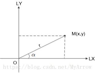
{ x = r ⋅ c o s ( α ) y = r ⋅ s i n ( α ) ( 公 式 1 ) \left\{ \begin{array}{c} x = r \cdot cos(\alpha) \\ y = r \cdot sin(\alpha) \end{array} \right. \qquad(公式1) {x=r⋅cos(α)y=r⋅sin(α)(公式1) - 激光点在 ( 公 式 1 ) (公式1) (公式1)的基础上再旋转了 β \beta β,则激光点 M ′ M' M′在激光坐标系中的坐标为 ( x ′ , y ′ ) (x', y') (x′,y′):
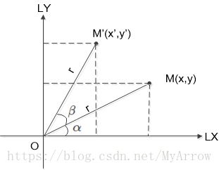
x ′ = r ⋅ c o s ( α + β ) = r ⋅ c o s ( α ) c o s ( β ) − r ⋅ s i n ( α ) s i n ( β ) x'=r \cdot cos(\alpha+\beta) = r \cdot cos(\alpha)cos(\beta) - r \cdot sin(\alpha) sin(\beta) x′=r⋅cos(α+β)=r⋅cos(α)cos(β)−r⋅sin(α)sin(β)
y ′ = r ⋅ s i n ( α + β ) = r ⋅ s i n ( α ) c o s ( β ) + r ⋅ c o s ( α ) s i n ( β ) y'=r \cdot sin(\alpha+\beta) = r \cdot sin(\alpha)cos(\beta) + r \cdot cos(\alpha) sin(\beta) y′=r⋅sin(α+β)=r⋅sin(α)cos(β)+r⋅cos(α)sin(β)
代入 公 式 ( 1 ) 公式(1) 公式(1),可得 公 式 ( 2 ) 公式(2) 公式(2):
{ x ′ = x ⋅ c o s ( β ) − y ⋅ s i n ( β ) y ′ = x ⋅ s i n ( β ) + y ⋅ c o s ( β ) ( 公 式 2 ) \left\{ \begin{array}{c} x' = x \cdot cos(\beta) - y \cdot sin(\beta) \\ y' = x \cdot sin(\beta) + y \cdot cos(\beta) \end{array} \right. \qquad(公式2) {x′=x⋅cos(β)−y⋅sin(β)y′=x⋅sin(β)+y⋅cos(β)(公式2)
矩阵表示为:
[ x ′ y ′ ] = [ c o s ( β ) − s i n ( β ) s i n ( β ) c o s ( β ) ] [ x y ] ( 公 式 2 ′ ) \begin{bmatrix} x' \\ y' \end{bmatrix} = \begin{bmatrix} cos(\beta) & -sin(\beta) \\ sin(\beta) & cos(\beta) \end{bmatrix} \begin{bmatrix} x \\ y \end{bmatrix} \qquad (公式2') [x′y′]=[cos(β)sin(β)−sin(β)cos(β)][xy](公式2′) - 一个旋转等价于同一个空间点在另一个不同坐标下对应位置的重新描述
- 设激光坐标系在世界坐标系中的位置为 ( L x , L y ) (L_x, L_y) (Lx,Ly),且相对于世界坐标系逆时针方向的旋转角度为 θ \theta θ,激光点在激光坐标系中的位置为 ( x , y ) ; (x,y); (x,y);则激光点N在世界坐标系中的坐标为 ( x w , y w ) (x_w, y_w) (xw,yw)( 注 : 无 论 在 哪 个 坐 标 系 中 , 点 N 在 空 间 中 的 位 置 始 终 保 持 不 变 \color{red}{注:无论在哪个坐标系中,点N在空间中的位置始终保持不变} 注:无论在哪个坐标系中,点N在空间中的位置始终保持不变):
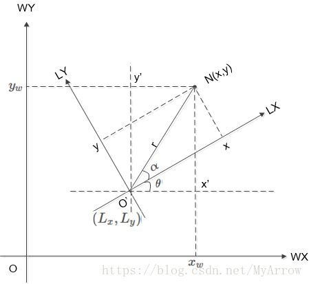
{ x ′ = r ⋅ c o s ( α + θ ) = r ⋅ c o s ( α ) c o s ( θ ) − r ⋅ s i n ( α ) s i n ( θ ) y ′ = r ⋅ s i n ( α + θ ) = r ⋅ s i n ( α ) c o s ( θ ) + r ⋅ c o s ( α ) s i n ( θ ) ⇒ \left\{ \begin{array}{c} x' = r \cdot cos(\alpha + \theta) = r \cdot cos(\alpha)cos(\theta) - r \cdot sin(\alpha)sin(\theta) \\ y' = r \cdot sin (\alpha + \theta) = r \cdot sin(\alpha)cos(\theta) + r \cdot cos(\alpha)sin(\theta) \end{array} \right. \Rightarrow {x′=r⋅cos(α+θ)=r⋅cos(α)cos(θ)−r⋅sin(α)sin(θ)y′=r⋅sin(α+θ)=r⋅sin(α)cos(θ)+r⋅cos(α)sin(θ)⇒
{ x ′ = x ⋅ c o s ( θ ) − y ⋅ s i n ( θ ) y ′ = x ⋅ s i n ( θ ) + y ⋅ c o s ( θ ) \left\{ \begin{array}{c} x' = x \cdot cos(\theta) - y \cdot sin(\theta) \\ y' = x \cdot sin(\theta) + y \cdot cos(\theta) \end{array} \right. {x′=x⋅cos(θ)−y⋅sin(θ)y′=x⋅sin(θ)+y⋅cos(θ)
{ x w = L x + x ′ y w = L y + y ′ \left\{ \begin{array}{c} x_w = L_x + x' \\ y_w = L_y + y' \end{array} \right. {xw=Lx+x′yw=Ly+y′ - ( 公 式 3 ) (公式3) (公式3)
{ x w = L x + x ⋅ c o s ( θ ) − y ⋅ s i n ( θ ) y w = L y + x ⋅ s i n ( θ ) + y ⋅ c o s ( θ ) ( 公 式 3 ) \left\{ \begin{array}{c} x_w = L_x + x \cdot cos(\theta) - y \cdot sin(\theta) \\ y_w = L_y + x \cdot sin(\theta) + y \cdot cos(\theta) \end{array} \right. \quad (公式3) {xw=Lx+x⋅cos(θ)−y⋅sin(θ)yw=Ly+x⋅sin(θ)+y⋅cos(θ)(公式3) - ( 公 式 3 ) (公式3) (公式3)矩阵表示
[ x w y w ] = [ L x L y ] + [ c o s ( θ ) − s i n ( θ ) s i n ( θ ) c o s ( θ ) ] [ x y ] ( 公 式 3 ′ ) \begin{bmatrix} x_w \\ y_w \end{bmatrix} = \begin{bmatrix} L_x \\ L_y \end{bmatrix} + \begin{bmatrix} cos(\theta) & -sin(\theta) \\ sin(\theta) & cos(\theta) \end{bmatrix} \begin{bmatrix} x \\ y \end{bmatrix} \qquad (公式3') [xwyw]=[LxLy]+[cos(θ)sin(θ)−sin(θ)cos(θ)][xy](公式3′)
2.1.1 根据在摄像机坐标系中的位置求在世界坐标系中的位置
- 对于2D坐标变换,设Camera的Pose为 ( t x , t y , θ ) (t_x, t_y, \theta) (tx,ty,θ),即其位置为(x,y), 方向为 θ \theta θ,它定义了Camera坐标系。
- 非齐次坐标系:
P w = R c P c + t c P_w = R_cP_c+t_c Pw=RcPc+tc- P c P_c Pc: P点在摄像机坐标系中的位置 [ x c , y c ] T [x_c,y_c]^T [xc,yc]T
- P w P_w Pw:P点在世界坐标系中的位置 [ x w , y w ] T [x_w,y_w]^T [xw,yw]T
- t c t_c tc:摄像机在世界坐标系中的位置 [ t x , t y ] T [t_x,t_y]^T [tx,ty]T
- R c R_c Rc:摄像机坐标系相对于世界坐标系的旋转矩阵:
R c = [ c o s ( θ ) − s i n ( θ ) s i n ( θ ) c o s ( θ ) ] R_c = \begin{bmatrix} cos(\theta) & -sin(\theta) \\ sin(\theta) & cos(\theta) \end{bmatrix} Rc=[cos(θ)sin(θ)−sin(θ)cos(θ)]
- 齐次坐标系:
P w = T r w P c P_w=T_{rw}P_c Pw=TrwPc- P c P_c Pc: P点在摄像机坐标系中的位置 [ x c , y c , 1 ] T [x_c,y_c, 1]^T [xc,yc,1]T
- P w P_w Pw:P点在世界坐标系中的位置 [ x w , y w , 1 ] T [x_w,y_w, 1]^T [xw,yw,1]T
- T r w T_{rw} Trw:从摄像机坐标系到世界坐标系的变换矩阵(包括平移和旋转)
T r w = [ c o s ( θ ) − s i n ( θ ) t x s i n ( θ ) c o s ( θ ) t y 0 0 1 ] T_{rw} = \begin{bmatrix} cos(\theta) & -sin(\theta) & t_x\\ sin(\theta) & cos(\theta) & t_y \\ 0 & 0 & 1 \end{bmatrix} Trw=⎣⎡cos(θ)sin(θ)0−sin(θ)cos(θ)0txty1⎦⎤
2.1.2 根据在世界坐标系中的位置求在摄像机坐标系中的位置
- 求 P c P_c Pc的公式(非齐次坐标系):
P c = R c − 1 ( P w − T c ) P_c=R_c^{-1}(P_w-T_c) Pc=Rc−1(Pw−Tc) - 求 P c P_c Pc的公式(齐次坐标系):
P c = T r w − 1 P w P_c = T_{rw}^{-1}P_w Pc=Trw−1Pw
2.2 3D变换
-
3D旋转表示方式:
- 旋转矩阵 R 3 × 3 R_{3 \times 3} R3×3(Eigen::Matrix3d)
- 旋转向量 R 3 × 1 R_{3 \times 1} R3×1(Eigen::AngleAxisd):使用旋转的角度和旋转轴向量(此向量必须为单位向量)定义
- 四元素 R 4 × 1 R_{4 \times 1} R4×1(Eigen::Quaterniond)
-
3D平移表示方式:
- 平移向量 t 3 × 1 t_{3 \times 1} t3×1:(Eigen::Vector3d)
-
变换矩阵(包括旋转和平移)
- T 4 × 4 T_{4 \times 4} T4×4:(Eigen::Isometry3d)
T r w = [ R 3 × 3 t 3 × 1 0 3 × 1 T 1 1 × 1 ] T_{rw} = \begin{bmatrix} R_{3 \times 3} & t_{3 \times 1}\\ 0_{3 \times 1}^T & 1_{1 \times 1} \end{bmatrix} Trw=[R3×303×1Tt3×111×1]
- T 4 × 4 T_{4 \times 4} T4×4:(Eigen::Isometry3d)
-
根据旋转R和平移t生成变换矩阵T
-
点P从摄像机坐标系变换到世界坐标系
P w = T r w P c P_w = T_{rw} P_c Pw=TrwPc -
点P从世界坐标系变换到摄像机坐标系
P c = T r w − 1 P w P_c = T_{rw}^{-1}P_w Pc=Trw−1Pw
2.3 Eigen旋转实现
- 旋转定义:归一化向量 ( n x , n y , n z ) (nx, ny, nz) (nx,ny,nz)表示旋转轴, θ \theta θ=M_PI/4表示旋转角(单位:辐度),以下的旋转变量均表示此旋转
2.3.1 AngleAxisd表示
AngleAxisd rot_v(M_PI/4, Vector3d(nx, ny, nz); // 需转换为matrix进行显示
2.3.2 Quaterniond表示
double A = (M_PI/4);
Quaterniond rot_q(cos(A/2), nx*sin(A/2), ny*sin(A/2), nz*sin(A/2));
// Quaterniondr的数据存储顺序:x,y,z,w; 初始化顺序:w,x,y,z
//第一种输出四元数的方式
cout << "Quaternion1" << endl << rot_q.coeffs() << endl;

//第二种输出四元数的方式
cout << rot_q.x() << endl << endl;
cout << rot_q.y() << endl << endl;
cout << rot_q.z() << endl << endl;
cout << rot_q.w() << endl << endl;
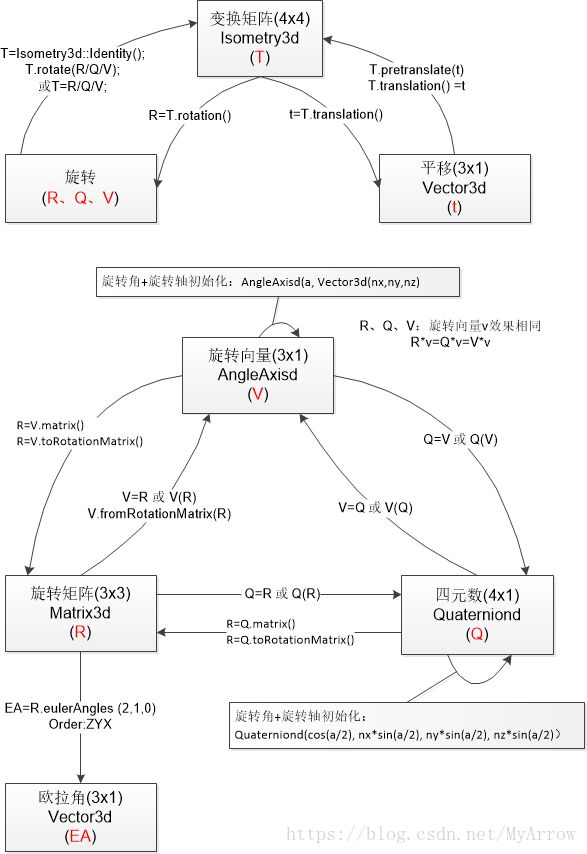
2.3.3 Quaterniond & AngleAxisd & Matrix3d相互转换
-
三维运动描述对应的 Eigen 数据类型总结
| 三维运动变换 | Eigen类 |
| ------------- | -----?
| 旋转矩阵(3 x 3) | Eigen::Matrix3d |
| 旋转向量(3 x 1 |Eigen::AngleAxisd |
| 欧拉角(3 x 1) |Eigen::Vector3d |
| 四元数 (4 x 1) | Eigen::Quaterniond |
| 欧氏变换矩阵(4 x 4 ) | Eigen::Isometry3d |
| 仿射变换(4 x 4) | Eigen::Affine3d |
| 射影变换(4 x 4) | Eigen::Perspective3d | -
变换表示转换图
- 旋转表示转换代码
#include
#include
#include
#include
#include
using namespace std;
using namespace Eigen;

int main()
{
    // The rotation definition:
    // rotation angle: M_PI/4
    // rotation axis: (0,0,1)
    AngleAxisd t_V(M_PI/4, Vector3d(0, 0, 1));
    Matrix3d t_R = t_V.matrix();
    Quaterniond t_Q(t_V);

    cout << "Matrix3d=\n" << t_R << endl;
    cout << "Quaterniond=\n" << t_Q.coeffs() << endl;
    cout << "Quaterniond Matrix=\n" << t_Q.matrix() << endl;
    cout << "AngleAxisd Matrix=\n" << t_V.matrix() << endl;


    //////////////////////////////////////////////
    ///  Init AngleAxisd
    //////////////////////////////////////////////
    AngleAxisd v1(M_PI / 4, Vector3d(0, 0, 1));
    cout << "AngleAxisd(1)=\n" << v1.matrix() << endl;

    AngleAxisd v2;
    v2.fromRotationMatrix(t_R);
    cout << "AngleAxisd(2)=\n" << v2.matrix() << endl;

    AngleAxisd v3;
    v3 = t_R;
    cout << "AngleAxisd(3)=\n" << v3.matrix() << endl;

    AngleAxisd v4(t_R);
    cout << "AngleAxisd(4)=\n" << v4.matrix() << endl;

    AngleAxisd v5;
    v5 = t_Q;
    cout << "AngleAxisd(5)=\n" << v5.matrix() << endl;

    AngleAxisd v6(t_Q);
    cout << "AngleAxisd(6)=\n" << v6.matrix() << endl;

    //////////////////////////////////////////////
    ///  Init Quanterniond
    //////////////////////////////////////////////
    //q=[cos(A/2),nx*sin(A/2),ny*sin(A/2),nz*sin(A/2)]
    // Angle M_PI/4, rotation axis: (0,0,1), that is z axis
    double angle = M_PI/4;
    Quaterniond Q1(cos(angle / 2),
                   0 * sin(angle / 2),
                   0 * sin(angle / 2),
                   1 * sin(angle / 2));
    //第一种输出四元数的方式
    cout << "Quaternion1" << endl << Q1.coeffs() << endl;

    //第二种输出四元数的方式
    cout << "output x,y,z,w:" << endl;
    cout << Q1.x() << endl;
    cout << Q1.y() << endl;
    cout << Q1.z() << endl;
    cout << Q1.w() << endl;

    Quaterniond Q2;
    Q2 = t_R;
    cout << "Quaternion2" << endl << Q2.coeffs() << endl;

    Quaterniond Q3(t_R);
    cout << "Quaternion3" << endl << Q3.coeffs() << endl;

    Quaterniond Q4;
    Q4 = t_V;
    cout << "Quaternion4" << endl << Q4.coeffs() << endl;

    Quaterniond Q5(t_V);
    cout << "Quaternion5" << endl << Q5.coeffs() << endl;

    //////////////////////////////////////////////
    ///  Init Rotation Matrix3d
    //////////////////////////////////////////////

    Matrix3d R1=Matrix3d::Identity();
    cout << "Rotation_matrix1" << endl << R1 << endl;

    Matrix3d R2;
    R2 = t_V.matrix();
    cout << "Rotation_matrix2" << endl << R2 << endl;

    Matrix3d R3;
    R3 = t_V.toRotationMatrix();
    cout << "Rotation_matrix3" << endl << R3 << endl;

    Matrix3d R4;
    R4 = t_Q.matrix();
    cout << "Rotation_matrix4" << endl << R4 << endl;

    Matrix3d R5;
    R5 = t_Q.toRotationMatrix();
    cout << "Rotation_matrix5" << endl << R5 << endl;

    //////////////////////////////////////////////
    ///  Init Euler angles
    //////////////////////////////////////////////
    Eigen::Vector3d euler_angles;
    euler_angles = t_R.eulerAngles (2,1,0); // ZYX order, that is:roll pitch yaw
    cout<< "M_PI/4=" << M_PI/4 << endl;
    cout<<"ZYX:yaw pitch roll = "<
2.3.4 把一个点变换到另一个点定义的坐标系中
- 两个点位于同一个坐标系(如世界坐标系)
- 点的位置为其对应坐标系的原点,点的旋转角为其坐标系的旋转角
#include
#include
#include
#include
#include
using namespace std;
using namespace Eigen;

int main()
{
    // P1w t=(1,0,0) yaw=M_PI/2
    // P2w t=(2,1,0) yaw=M_PI/2
    // The position of P2w in P1w frame is (1, -1, 0)

    ////////////////////////////////////////////////////////////////////////
    /// set p1w as frame, slove the position of point P2w in the p1w frame
    /// ////////////////////////////////////////////////////////////////////
    AngleAxisd rot_v1 = AngleAxisd(M_PI/2, Vector3d(0,0,1));
    cout << "rotation=\n" << rot_v1.matrix() << endl;

    Vector3d t1 = Vector3d(1,0,0);

    // T1 is the transfrom from camera frame to world frame
    // Tcw: T1
    // Pw = Tcw * Pc = T1 * Pc
    // Pc = T1^(-1) * Pw
    Isometry3d  T1 = Isometry3d::Identity();
    //T1 = rot_v1;
    T1.rotate(rot_v1);

    cout << "T1=\n" << T1.matrix() << endl;
    T1.pretranslate(t1);
    cout << "T1+T=\n" << T1.matrix() << endl;

    Vector3d p2w = Vector3d(2,1,0);
    Vector3d p2c = T1.inverse()*p2w;

    cout << "p2c=\n" << p2c << endl;

    cout << "(1,0,0) world position=\n" << T1 * Vector3d(1,0,0) << endl;

    return 0;
}
3. 点乘与叉乘的几何含义
3.1 点乘
- 定义:
a = [ a 1 , a 2 , ⋯ , a n ] T b = [ b 1 , b 2 , ⋯ , b n ] T a=[a_1,a_2, \cdots, a_n]^T \quad b=[b_1, b_2, \cdots, b_n]^T a=[a1,a2,⋯,an]Tb=[b1,b2,⋯,bn]T
a ⋅ b = a T b = ∣ a ∣ ⋅ ∣ b ∣ ⋅ c o s ( θ ) θ 为 向 量 a 与 b 的 夹 角 a \cdot b = a^Tb= \vert a \vert \cdot \vert b \vert \cdot cos(\theta) \quad \theta 为向量a与b的夹角 a⋅b=aTb=∣a∣⋅∣b∣⋅cos(θ)θ为向量a与b的夹角 - 输出值:标量
- 几何意义:
- 是一个向量和它在另一个向量上的投影长度的乘积;
- 反映两个向量的“相似度”,两个向量越“相似”,它们的点乘越大;
- 可以计算向量a和向量b之间的夹角;
- 可以步判断这两个向量是否是同一方向,是否正交(也就是垂直)等方向关系,具体对应关系为:
- a ⋅ b > 0 a \cdot b>0 a⋅b>0:方向基本相同,夹角在0°到90°之间
- a ⋅ b = 0 a \cdot b=0 a⋅b=0:正交,相互垂直 ,夹角为90°
- a ⋅ b < 0 a \cdot b<0 a⋅b<0:方向基本相反,夹角在90°到180°之间
3.2 叉乘
4. 其它资料
- 3D坐标变换
- 四元素
- Eigen旋转表示及运算实例
- C++矩阵库 Eigen 快速入门
- Eigen官方手册