Fourier Transform Intro - Oscillation frequency vs Angular frequency Expression
http://mathworld.wolfram.com/FourierTransform.html
Fourier Transform
![]()
![]()
The Fourier transform is a generalization of the complex Fourier series in the limit as  . Replace the discrete
 with the continuous
 while letting
 . Then change the sum to anintegral, and the equations become
 |
 |
 |
(1)
|
 |
 |
 |
(2)
|
Here,
 |
 |
](http://img.e-com-net.com/image/info5/5874541415b146c194f25f37dc9f41f7.jpg) |
(3)
|
 |
 |
 |
(4)
|
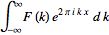
is called the forward ( ) Fourier transform, and
 |
 |
](http://img.e-com-net.com/image/info5/1c1c26da4db24a729947a1a4fac03c5a.jpg) |
(5)
|
 |
 |
 |
(6)
|
is called the inverse ( ) Fourier transform. The notation
](http://img.e-com-net.com/image/info5/052a6f2f27cc4b018cb27af1463f9eb2.jpg) is introduced in Trott (2004, p. xxxiv), and
is introduced in Trott (2004, p. xxxiv), and and
and are sometimes also used to denote the Fourier transform and inverse Fourier transform, respectively (Krantz 1999, p. 202).
Note that some authors (especially physicists) prefer to write the transform in terms of angular frequency instead of the oscillation frequency
 . However, this destroys the symmetry, resulting in the transform pair
 |
 |
![F[h(t)]](http://img.e-com-net.com/image/info5/9f2f0d50d447482291425b40bb72719d.jpg) |
(7)
|
 |
 |
 |
(8)
|
 |
 |
![F^(-1)[H(omega)]](http://img.e-com-net.com/image/info5/97a47d411f004739b9d1fafe21d533c5.jpg) |
(9)
|
 |
 |
 |
(10)
|
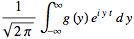
To restore the symmetry of the transforms, the convention
 |
 |
![F[f(t)]](http://img.e-com-net.com/image/info5/f46dc0455da44adbadd1f9b2f769ce0e.jpg) |
(11)
|
 |
 |
 |
(12)
|
 |
 |
![F^(-1)[g(y)]](http://img.e-com-net.com/image/info5/eb88ca88f9df4670ac74960db4734f58.jpg) |
(13)
|
 |
 |
 |
(14)
|
is sometimes used (Mathews and Walker 1970, p. 102).
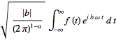
In general, the Fourier transform pair may be defined using two arbitrary constants and
and as
as
 |
 |
 |
(15)
|
 |
 |
 |
(16)
|
The Fourier transform  of a function
 is implemented theWolfram Language asFourierTransform[f,x,k], and different choices of
  and
and can be used by passing the optionalFourierParameters->
  a,b
a,b option. By default, theWolfram Language takesFourierParameters as
 . Unfortunately, a number of other conventions are in widespread use. For example,
 is used in modern physics,
 is used in pure mathematics and systems engineering,
 is used in probability theory for the computation of thecharacteristic function,
 is used in classical physics, and
 is used in signal processing. In this work, following Bracewell (1999, pp. 6-7),it is always assumed that
 and
and unless otherwise stated. This choice often results in greatly simplified transforms of common functions such as 1,
 , etc.
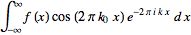
Since any function can be split up into even and odd portions  and
and ,
,
 |
 |
![1/2[f(x)+f(-x)]+1/2[f(x)-f(-x)]](http://img.e-com-net.com/image/info5/2d26c1ca7fb64c60af2abf8ba1898a72.gif) |
(17)
|
 |
 |
 |
(18)
|
a Fourier transform can always be expressed in terms of the Fourier cosine transform and Fourier sine transform as
=int_(-infty)^inftyE(x)cos(2pikx)dx-iint_(-infty)^inftyO(x)sin(2pikx)dx.](http://img.e-com-net.com/image/info5/33c0c63dfcaa4dfb88e89aaaa623ff58.gif) |
(19)
|
A function  has a forward and inverse Fourier transform such that
![f(x)={int_(-infty)^inftye^(2piikx)[int_(-infty)^inftyf(x)e^(-2piikx)dx]dk for f(x) continuous at x; 1/2[f(x_+)+f(x_-)] for f(x) discontinuous at x,](http://img.e-com-net.com/image/info5/895e8be808c64509b06512a270027a15.gif) |
(20)
|
provided that
1.  exists.
2. There are a finite number of discontinuities.
3. The function has bounded variation. A sufficient weaker condition is fulfillment of the Lipschitz condition
(Ramirez 1985, p. 29). The smoother a function (i.e., the larger the number of continuousderivatives), the more compact its Fourier transform.
The Fourier transform is linear, since if  and
and have Fourier transforms
 and
and , then
![int[af(x)+bg(x)]e^(-2piikx)dx](http://img.e-com-net.com/image/info5/7b76ed26482849dbb0e1976f333f5766.jpg) |
 |
 |
(21)
|
 |
 |
 |
(22)
|
Therefore,
![F[af(x)+bg(x)]](http://img.e-com-net.com/image/info5/4b0a358659524944a617d986b6169b6b.jpg) |
 |
![aF[f(x)]+bF[g(x)]](http://img.e-com-net.com/image/info5/a9289722e8264e6ca3cb05c956e9623a.jpg) |
(23)
|
 |
 |
 |
(24)
|
The Fourier transform is also symmetric since ](http://img.e-com-net.com/image/info5/4455d1000bd84befa36f9645881c26d3.jpg) implies
implies](http://img.e-com-net.com/image/info5/4ea4c6ba6bdd46bc960f0acc51d64063.jpg) .
.
Let  denote theconvolution, then the transforms of convolutions of functions have particularly nice transforms,
![F[f*g]](http://img.e-com-net.com/image/info5/26436b7f0ab541a488a7c73b4eb91c2e.jpg) |
 |
![F[f]F[g]](http://img.e-com-net.com/image/info5/91c61f8d97294d6d81848a9edf2447f2.jpg) |
(25)
|
![F[fg]](http://img.e-com-net.com/image/info5/cc19c5f7cea44ba892cf326d9a895845.jpg) |
 |
![F[f]*F[g]](http://img.e-com-net.com/image/info5/eec938d1f8c54aa79c8ab6c727b2f095.jpg) |
(26)
|
![F^(-1)[F(f)F(g)]](http://img.e-com-net.com/image/info5/4ad7ed0e17694be1802c92e327304962.jpg) |
 |
 |
(27)
|
![F^(-1)[F(f)*F(g)]](http://img.e-com-net.com/image/info5/7387ff00f573481dbfde8c47203342ad.jpg) |
 |
 |
(28)
|
The first of these is derived as follows:
![F[f*g]](http://img.e-com-net.com/image/info5/b46b9170ca6b4f088ed04320c99cb710.jpg) |
 |
 |
(29)
|
 |
 |
![int_(-infty)^inftyint_(-infty)^infty[e^(-2piikx^')f(x^')dx^'][e^(-2piik(x-x^'))g(x-x^')dx]](http://img.e-com-net.com/image/info5/068b4d5af8d4443eb112559f12b9d5d2.gif) |
(30)
|
 |
 |
![[int_(-infty)^inftye^(-2piikx^')f(x^')dx^'][int_(-infty)^inftye^(-2piikx^(''))g(x^(''))dx^('')]](http://img.e-com-net.com/image/info5/a38b5b0f229348819de384925dd3a03b.gif) |
(31)
|
 |
 |
![F[f]F[g],](http://img.e-com-net.com/image/info5/28320e34eddc4c21ab7c7c6c79a3aa1c.jpg) |
(32)
|
where  .
.
There is also a somewhat surprising and extremely important relationship between theautocorrelation and the Fourier transform known as theWiener-Khinchin theorem. Let =F(k)](http://img.e-com-net.com/image/info5/1984aa84aea84e6d83a511d8b460dbbf.jpg) , and
, and denote thecomplex conjugate of
 , then the Fourier transform of theabsolute square of
 is given by
=int_(-infty)^inftyf^_(tau)f(tau+x)dtau.](http://img.e-com-net.com/image/info5/1f514475eaa944b4bb0b4b90ff7849d4.gif) |
(33)
|
The Fourier transform of a derivative  of a function
 is simply related to the transform of the function
 itself. Consider
=int_(-infty)^inftyf^'(x)e^(-2piikx)dx.](http://img.e-com-net.com/image/info5/edf9fe1cf8624e0997d81c4880373fe4.gif) |
(34)
|
Now use integration by parts
![intvdu=[uv]-intudv](http://img.e-com-net.com/image/info5/27d3a2e8917f42829accd45d3818288c.gif) |
(35)
|
with
 |
 |
 |
(36)
|
 |
 |
 |
(37)
|
and
 |
 |
 |
(38)
|
 |
 |
 |
(39)
|
then
=[f(x)e^(-2piikx)]_(-infty)^infty-int_(-infty)^inftyf(x)(-2piike^(-2piikx)dx).](http://img.e-com-net.com/image/info5/f183bfc2a38d437ab3613755424cdf82.gif) |
(40)
|
The first term consists of an oscillating function times  . But if the function is bounded so that
 |
(41)
|
(as any physically significant signal must be), then the term vanishes, leaving
](http://img.e-com-net.com/image/info5/b1163bd509574a69933956c248a54068.jpg) |
 |
 |
(42)
|
 |
 |
.](http://img.e-com-net.com/image/info5/1289146503ee4aec94af972cca50c5da.jpg) |
(43)
|
This process can be iterated for the  thderivative to yield
=(2piik)^nF_x[f(x)](k).](http://img.e-com-net.com/image/info5/7fef7107d76d4d468a24f91b94a96391.gif) |
(44)
|
The important modulation theorem of Fourier transforms allows ](http://img.e-com-net.com/image/info5/f1f5c87e1ab6413392a8a4e630b1cc11.jpg) to be expressed in terms of
to be expressed in terms of=F(k)](http://img.e-com-net.com/image/info5/512d3603eb984b2883235286cdb2c287.jpg) as follows,
as follows,
](http://img.e-com-net.com/image/info5/703ec78ef0e0455889cadbf63f8f484a.jpg) |
 |
 |
(45)
|
 |
 |
 |
(46)
|
 |
 |
 |
(47)
|
 |
 |
![1/2[F(k-k_0)+F(k+k_0)].](http://img.e-com-net.com/image/info5/453cb94c97a046c8b99b2589af83b7c3.gif) |
(48)
|
Since the derivative of the Fourier transform is given by
=int_(-infty)^infty(-2piix)f(x)e^(-2piikx)dx,](http://img.e-com-net.com/image/info5/b5885e209ca842cf9e59a036ca7284f1.gif) |
(49)
|
it follows that
 |
(50)
|
Iterating gives the general formula
 |
 |
 |
(51)
|
 |
 |
 |
(52)
|
The variance of a Fourier transform is
 |
(53)
|
and it is true that
 |
(54)
|
If  has the Fourier transform
=F(k)](http://img.e-com-net.com/image/info5/d027d2bd2ce242d286f2742a9af21333.jpg) , then the Fourier transform has the shift property
, then the Fourier transform has the shift property
 |
 |
 |
(55)
|
 |
 |
 |
(56)
|
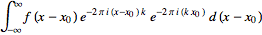
so  has the Fourier transform
=e^(-2piikx_0)F(k).](http://img.e-com-net.com/image/info5/28c3869d313146e9b0d3446946c71eec.jpg) |
(57)
|
If  has a Fourier transform
=F(k)](http://img.e-com-net.com/image/info5/89ef07da6da5464287d670bed8f47d16.jpg) , then the Fourier transform obeys a similarity theorem.
, then the Fourier transform obeys a similarity theorem.
 |
(58)
|
so  has the Fourier transform
=|a|^(-1)F(k/a).](http://img.e-com-net.com/image/info5/e590cea5c1464b9e92d30c94bbff7a90.jpg) |
(59)
|
The "equivalent width" of a Fourier transform is
 |
 |
 |
(60)
|
 |
 |
 |
(61)
|
The "autocorrelation width" is
 |
 |
![(int_(-infty)^inftyf*f^_dx)/([f*f^_]_0)](http://img.e-com-net.com/image/info5/391aab109ad14d5ab4c98d0cc5742387.gif) |
(62)
|
 |
 |
 |
(63)
|
where  denotes thecross-correlation of
 and
and and
and is thecomplex conjugate.
Any operation on  which leaves itsarea unchanged leaves
 unchanged, since
=F(0).](http://img.e-com-net.com/image/info5/13cfc293805e4ead921cff940ddbe1cb.gif) |
(64)
|
The following table summarized some common Fourier transform pairs.
| function |  |
](http://img.e-com-net.com/image/info5/1d4edd9b52e14cd48741314b6be0d186.jpg) |
| Fourier transform--1 | 1 |  |
| Fourier transform--cosine |  |
![1/2[delta(k-k_0)+delta(k+k_0)]](http://img.e-com-net.com/image/info5/a711d189e2cc424b8f1e0ca468d0142a.gif) |
| Fourier transform--delta function |  |
 |
| Fourier transform--exponential function |  |
 |
| Fourier transform--Gaussian |  |
 |
| Fourier transform--Heaviside step function |  |
![1/2[delta(k)-i/(pik)]](http://img.e-com-net.com/image/info5/8bc638e43c6f4975b2b131c12ac61f2e.jpg) |
| Fourier transform--inverse function |  |
![i[1-2H(-k)]](http://img.e-com-net.com/image/info5/8a39dd9e968a47468a138d23e9286b8b.jpg) |
| Fourier transform--Lorentzian function |  |
 |
| Fourier transform--ramp function |  |
 |
| Fourier transform--sine |  |
![1/2i[delta(k+k_0)-delta(k-k_0)]](http://img.e-com-net.com/image/info5/5132ed6a836d4262b61b03dc68c87731.gif) |
In two dimensions, the Fourier transform becomes
 |
 |
 |
(65)
|
 |
 |
 |
(66)
|
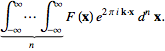
Similarly, the  -dimensional Fourier transform can be defined for
 ,
, by
by
 |
 |
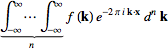 |
(67)
|
 |
 |
 |
(68)
|