高斯牛顿法,LM法
Gauss–Newton algorithm
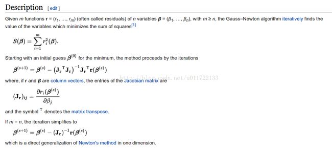
应用场景:The Gauss–Newton algorithm is used to solve non-linear least squares problems
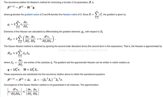
高斯牛顿法的推导来自于牛顿法,Wiki的数学推导确实很清楚:
Derivation from Newton's method

Levenberg–Marquardt algorithm
![]()
(xi,yi)是一组观测数据,xi, yi是实数;β是我们要优化的变量,假设为n*1维:增量δ(向量)通过下式确定:
The sum of squares at its minimum has a zero gradient with respect to β. The above first-order approximation of gives
or in vector notation,
Taking the derivative of with respect to δ and setting the result to zero gives
- 实数对向量求导
where is the Jacobian matrix,(m*n维) whose i-th row equals , and where (m*1维)and (m*1维)are vectors with i-th component and respectively. This is a set of linear equations, which can be solved for δ.
从这看到增量的求解是这样的过程:
目标函数是, 对自变量 β 产生一个增量δ,新的目标函数S(β+δ)的近似表达式 对增量 δ求导,令导数为0得到的。
这么求增量 β的原因是不是这么理解:
假设 β ^是使得最小的值,如何求得最优解 β ^呢? 换句话说,在初值β0的基础上,如何确定一个增量δ,使得最小?
逆向考虑:假设我们已经得到了这个增量δ,那必然 S’(β0+δ) =0。
现在的问题是如何求δ,即 δ是未知量。 而 δ又满足 S’(β0+δ) =0,要求 δ,那只有S(β0+δ)对 δ求导,令其导数为0得到。
Levenberg's contribution is to replace this equation by a "damped version",
where I is the identity matrix, giving as the increment δ to the estimated parameter vector β.
猜测可能需要计算 || S(β+δ)-S(β) || 是否超过某一个阈值. If 超过阈值,减小λ ;else,增大λ
The (non-negative) damping factor λ is adjusted at each iteration. If reduction of S is rapid, a smaller value can be used, bringing the algorithm closer to the Gauss–Newton algorithm, whereas if an iteration gives insufficient reduction in the residual, λ can be increased, giving a step closer to the gradient-descent direction.
If either the length of the calculated step δ or the reduction of sum of squares from the latest parameter vector β + δ fall below predefined limits, iteration stops, and the last parameter vector β is considered to be the solution.
Levenberg's algorithm has the disadvantage thatif the value of damping factor λ is large, inverting JTJ + λI is not used at all. Marquardt provided the insight that we can scale each component of the gradient according to the curvature(曲率), so that there is larger movement along the directions where the gradient is smaller. This avoids slow convergence in the direction of small gradient. Therefore, Marquardt replaced the identity matrix I with the diagonal matrix consisting of the diagonal elements of JTJ, resulting in the Levenberg–Marquardt algorithm:
L-M方法的一些实现库,全部的见wiki
The GNU Scientific Library has a C interface to MINPACK.
C/C++ Minpack includes the Levenberg–Marquardt algorithm
levmar is an implementation in C/C++ with support for constraints
sparseLM is a C implementation aimed at minimizing functions with large, arbitrarily sparse Jacobians. Includes a MATLAB MEX interface
InMin library contains a C++ implementation of the algorithm based on the eigen C++ linear algebra library. It has a pure C-language API as well as a Python binding
ceres is a non-linear minimisation library with an implementation of the Levenberg–Marquardt algorithm. It is written in C++ and uses eigen
ALGLIB has implementations of improved LMA in C# / C++ / Delphi / Visual Basic. Improved algorithm takes less time to converge and can use either Jacobian or exact Hessian.
